Difference between revisions of "Composite IPR"
(Created page with "__TOC__ == Composite Inflow Performance Relationship== thumb|right|300px|3 Phase IPR Curve <ref name=KermitBrown1984/> 3 Phase IPR calculat...") |
(→Nomenclature) |
||
| (4 intermediate revisions by the same user not shown) | |||
| Line 1: | Line 1: | ||
__TOC__ | __TOC__ | ||
== Composite Inflow Performance Relationship== | == Composite Inflow Performance Relationship== | ||
| − | [[File: | + | [[File:Composite IPR Curve.png|thumb|right|300px|Composite IPR Curve <ref name=KermitBrown1984/>]] |
| − | [[ | + | [[Composite IPR]] calculates [[IPR]] curve for oil wells producing water at various [[WCUT | watercuts]]. |
| − | [[ | + | [[Composite IPR]] equation was derived by Petrobras based on combination of [[Vogel's IPR]] equation for oil flow and constant productivity for water flow <ref name=KermitBrown1984/>. |
| − | [[ | + | [[Composite IPR]] curve is determined geometrically from those equations considering the fractional flow of oil and water <ref name=KermitBrown1984/>. |
==Math and Physics== | ==Math and Physics== | ||
| Line 41: | Line 41: | ||
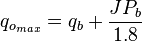
:<math> q_{o_{max}}=q_b+\frac{JP_b}{1.8}</math><ref name=KermitBrown1984/> | :<math> q_{o_{max}}=q_b+\frac{JP_b}{1.8}</math><ref name=KermitBrown1984/> | ||
| − | ==[[ | + | ==[[Composite IPR]] calculation example== |
| − | [[File:3 Phase IPR calculation example.png|thumb|right|400px| Figure.1 [https://www.pengtools.com/pqPlot?paramsToken=73eca3000d5f28d661700c874ebcf1f1 | + | [[File:3 Phase IPR calculation example.png|thumb|right|400px| Figure.1 [https://www.pengtools.com/pqPlot?paramsToken=73eca3000d5f28d661700c874ebcf1f1 Composite IPR calculation example]]] |
Following the example problem #21, page 33 <ref name=KermitBrown1984 />: | Following the example problem #21, page 33 <ref name=KermitBrown1984 />: | ||
===Given:=== | ===Given:=== | ||
| Line 52: | Line 52: | ||
===Calculate:=== | ===Calculate:=== | ||
| − | Determine the [[ | + | Determine the [[Composite IPR]] curves for F<sub>w</sub>=0, 0.25, 0.5, 0.75, and 1. |
| + | |||
===Solution:=== | ===Solution:=== | ||
The problem was run through [[:Category:PQplot | PQplot]] software for different values of watercut. | The problem was run through [[:Category:PQplot | PQplot]] software for different values of watercut. | ||
| − | Result [[ | + | Result [[Composite IPR]] curves are shown on '''Fig.1'''. Points indicate results obtained by Brown <ref name=KermitBrown1984 />. |
| − | The [[:Category:PQplot|PQplot]] model from this example is available online by the following link: [https://www.pengtools.com/pqPlot?paramsToken=73eca3000d5f28d661700c874ebcf1f1 | + | The [[:Category:PQplot|PQplot]] model from this example is available online by the following link: [https://www.pengtools.com/pqPlot?paramsToken=73eca3000d5f28d661700c874ebcf1f1 Composite IPR calculation example] |
== Nomenclature == | == Nomenclature == | ||
| Line 65: | Line 66: | ||
:<math> F_o </math> = oil fraction, fraction | :<math> F_o </math> = oil fraction, fraction | ||
:<math> F_w </math> = water fraction, fraction | :<math> F_w </math> = water fraction, fraction | ||
| − | :<math> J </math> = productivity index, stb/d/psia | + | :<math> J </math> = oil productivity index, stb/d/psia |
:<math> P </math> = pressure, psia | :<math> P </math> = pressure, psia | ||
:<math> q </math> = flowing rate, stb/d | :<math> q </math> = flowing rate, stb/d | ||
| Line 93: | Line 94: | ||
:[[IPR]]<BR/> | :[[IPR]]<BR/> | ||
:[[Vogel's IPR]]<BR/> | :[[Vogel's IPR]]<BR/> | ||
| + | :[[3 Phase IPR]]<BR/> | ||
:[[Darcy's law]]<BR/> | :[[Darcy's law]]<BR/> | ||
{{#seo: | {{#seo: | ||
| − | |title= | + | |title=Composite IPR curve |
|titlemode= replace | |titlemode= replace | ||
|keywords=Inflow Performance Relationship, nodal analysis, IPR curve, IPR calculator | |keywords=Inflow Performance Relationship, nodal analysis, IPR curve, IPR calculator | ||
| − | |description= | + | |description= Composite inflow performance relationship for oil wells producing water. |
}} | }} | ||
[[Category:PQplot]] | [[Category:PQplot]] | ||
Latest revision as of 18:45, 13 June 2023
Contents
Composite Inflow Performance Relationship

Composite IPR calculates IPR curve for oil wells producing water at various watercuts.
Composite IPR equation was derived by Petrobras based on combination of Vogel's IPR equation for oil flow and constant productivity for water flow [1].
Composite IPR curve is determined geometrically from those equations considering the fractional flow of oil and water [1].
Math and Physics
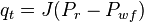
Total flow rate equations:
For Pb < Pwf < Pr
For pressures between reservoir pressure and bubble point pressure:
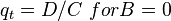
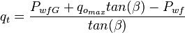
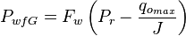
For PwfG < Pwf < Pb
For pressures between the bubble point pressure and the flowing bottom-hole pressures:
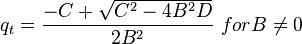
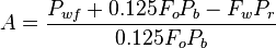
where:
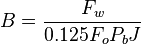
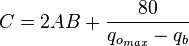
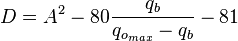
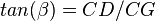
For 0 < Pwf < PwfG
where:

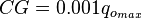
And
Composite IPR calculation example

Following the example problem #21, page 33 [1]:
Given:
 = 2550 psi
 = 2100 psi
Test data:
 = 2300 psi
 = 500 b/d
Calculate:
Determine the Composite IPR curves for Fw=0, 0.25, 0.5, 0.75, and 1.
Solution:
The problem was run through PQplot software for different values of watercut.
Result Composite IPR curves are shown on Fig.1. Points indicate results obtained by Brown [1].
The PQplot model from this example is available online by the following link: Composite IPR calculation example
Nomenclature
 = calculation variables
 = oil fraction, fraction
 = water fraction, fraction
 = oil productivity index, stb/d/psia
 = pressure, psia
 = flowing rate, stb/d
Subscripts
- b = at bubble point
- max = maximum
- o = oil
- r = reservoir
- t = total
- wf = well flowing bottomhole pressure
- wfG = well flowing bottomhole pressure at point G