Category: OptiFracMS
Contents
- 1 Multistage Fracturing Optimization Software
- 2 Typical applications
- 3 Math & Physics
- 4 Multistage Fracturing Design Optimization Type Curve
- 5 Physical Constraints of the Multistage Fracturing
- 6 Economic optimization of the Multistage Fracturing
- 7 Multistage Fracturing Optimization Flow Diagram
- 8 Multistage Fracturing Optimization Workflow
- 9 Hydraulic Fracturing Design Optimization - Bakken Case Study
- 10 Main optiFracMS features
- 11 Nomenclature
- 12 References
Multistage Fracturing Optimization Software
optiFracMS is a software to optimize the number of hydraulic fractures in horizontal well [1].
For the given set of reservoir properties and the proppant mass optiFracMS calculates optimal number of transverse hydraulic fractures and required fractures geometry to maximize well productivity index.
optiFracMS is available online at www.pengtools.com.
Typical applications
- Multistage Fracturing Design in horizontal wells in tight oil and gas reservoirs
- Calculation of the optimal number of fractures for a horizontal well with multiple transverse hydraulic fractures
- Number of fractures, n.
- Calculation of the optimal fractures geometry and conductivity:
- Dimensionless Fracture conductivity, CfD .
- Fracture half length, xf .
- Fracture width, wf .
- Fracture penetration, Ix .
- Calculation of the maximum productivity of a horizontal well with multiple transverse hydraulic fractures
- Dimensionless productivity index, JD .
- Application of the practical constrains to the multistage fracturing design: choke skin and minimum fracture width.
- Multistage Post fracture performance reviews
- Find out how far your well's productivity from where it should be (from the optimum)
- Multistage Fracturing Sensitivity Studies and Benchmarking
Math & Physics

 - technical potential for multistage fracturing [1],
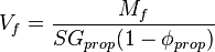
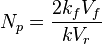 - proppant number,
 - penetration ratio,
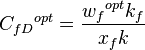
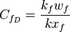 - dimensionless fracture conductivity,
Multistage Fracturing Design Optimization Type Curve
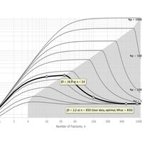
The type curves show multistage fracturing dimensionless productivity index, JD , at pseudo-steady state as a function of number of fractures, n, and proppant number, Np, for a horizontal well with multiple transverse hydraulic fractures in a square drainage area.
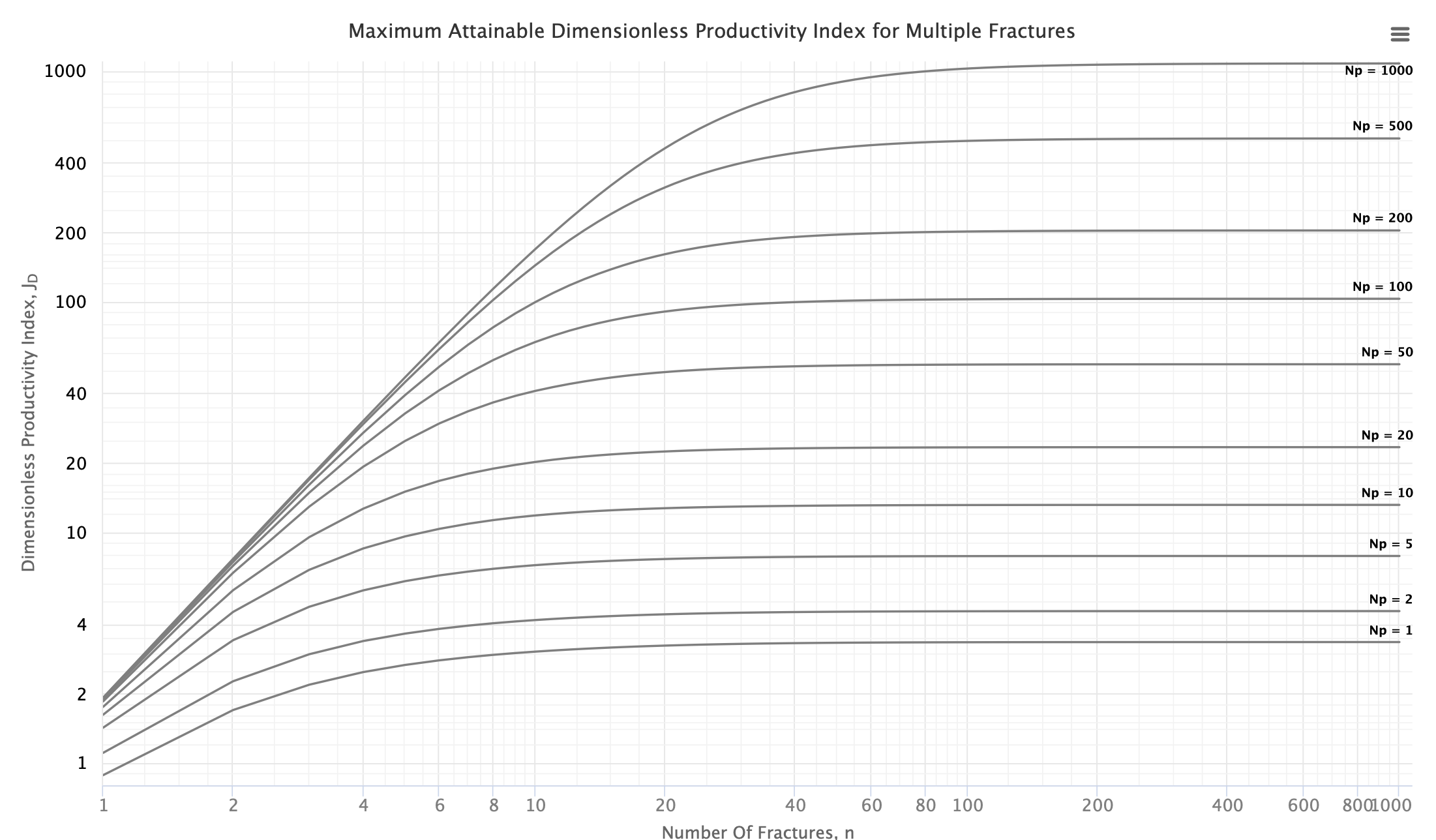
Type Curves were obtained, through 28,000 runs with direct boundary element (DBE) method [1].
For the given proppant number, Np, the more fractures that are created the higher the well JD. This is achieved by increasing the number of fractures, n, at the expense of individual fracture half-length and/or width. However, at some point, the additional increase in the number of fractures will result in fractures that are too slim to be practical. Such constrain is addressed below.
These type curves are also applicable for the case of rectangular (nonsquare) drainage areas.
Modification to rectangular (nonsquare) drainage areas

To design a multistage fracture in a rectangular area with dimensions Xe x Ye:
1. Calculate the proppant mass allocated for one square:
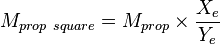
2. Run the multistage fracture design for the square area: Xe x Xe with the proppant mass Mpropsquare to get:


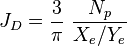
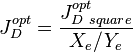
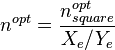
3. Calculae JDopt and nopt for the rectangular area Xe x Ye:
Type curve lookup table
The result of 28,000 runs with direct boundary element (DBE) method is a table which relates main parameters as follows:
| Np | n | JDmax | Ixopt | Ix = 0.01 | Ix = 0.02 | ... | Ix = 1 |
|---|---|---|---|---|---|---|---|
| 1 | 1 | 0.88 | 0.61 | JD = 0.23 | 0.25 | ... | 0.80 |
| 1 | 2 | 1.7 | 0.51 | 0.44 | 0.52 | ... | 1.38 |
| ... | ... | ... | ... | ... | ... | ... | ... |
| 1000 | 1000 | 989.6 | 0.99 | 1.88 | 1.97 | ... | 984.09 |
This table is used to lookup values for multistage fracturing design optimization process.
Physical Constraints of the Multistage Fracturing
Choke skin
Choke skin is defined as the additional pressure loss because of convergence of flow in the vertical fracture to the horizontal wellbore.
Choke skin can be calculated as follows:
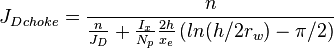
The effect of choke skin does not change the behavior of JD vs. n type curve, but but reduces maximum JD by as much as 9% [1].

The correction factor as a function of n for xe/h = 65 and h/rw=250 [1].
The choke skin effect increases with the number of fractures, however this dependence finally flattens out.
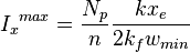
Minimum fracture width constraint
To maintain the fracture permeability kf, at least three proppant grains of width are required [2].
To account for this practical requirement, the deviation from the technical optimum will be required[2]. Instead of further decreasing the fracture width, the only possible option for a further increase in the number of fractures will be to decrease each fracture half-length. This will result in suboptimal performance of each fracture and, hence, suboptimal performance of the whole system in comparison to the ideal case without the minimum practical fracture width.
Requirement of the practical minimum-width constraint converted to maximum practical penetration ratio, which sets the limit to JD:

Effect of applying minimum fracture width constraint to the type curves (k=0.01md, kf=100d, xe=1609m, wmin=2.1mm) [1].
For the given proppant number, Np (above 20), there is an optimal number of fractures, n, with maximum well JD. Further increase in the number of fractures, n, will sharply decrease JD, because the fracture length is reduced to maintain the minimum width constraint for ever-reducing proppant volume per fracture.
Economic optimization of the Multistage Fracturing
The optimal number of stages seen above are strictly technical and do not include any cost and money value effects. Instead, these type curves can be used for the process of further economic optimization. Knowing the functional relationship between JD, NP, and n, and the cost of adding NP and n, the economic optimum can more readily be calculated [1].
Multistage Fracturing Optimization Flow Diagram

Multistage Fracturing Optimization Workflow
1. Calculate the Np:
 the volume of the reservoir
 the fracture permeability
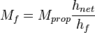 the proppant mass in the pay zone
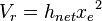
 the fracture volume in the pay zone
- the proppant number
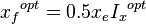
2. Apply the minimum fracture width constraint to calculate Ixopt and wfopt.
3. Read JDopt and nopt from the Multistage Fracturing Design Optimization Type Curve
3. Calculate single fracture parameters using the optiFrac :
Hydraulic Fracturing Design Optimization - Bakken Case Study

To illustrate the capabilities of the optiFracMS software a case study was prepared.
The goal of the study is to optimize a fracturing design for a Bakken formation.
Two fracture design cases were considered:
- Operating company fracture design based on a Big Data application
- optiFracMS optimized fracturing design
For the both cases a production forecast was calculated and cumulative oil production was compared.
Optimized fracture design case predicts 61% more cumulative oil in the first year of well production.
Read more: Hydraulic Fracturing Design Optimization - Bakken Case Study.
Main optiFracMS features
- Plot of JD as a function of n and Np as parameter.
- Plot of JD as a function of Np showing the width constraint influence.
- Plot of JD and wf as a function of n for the given Np .
- Plot of JD as a function of CfD for the given n.
- Design optimization curves which corresponds to the maximum JD values for different Np and n.
- Optimum number of fractures n and well JD.
- Practical constrains envelope – minimum fracture width and choke skin effect.
- Sensitivity for the different parameters: n, Xf, Ix, CfD, wf.
- Hydraulic fracturing proppant catalog with the predefined proppant properties.
- Save and share models with colleagues
- Last saved model on current computer and browser is automatically opened
- Metric and US oilfield units
- Save as image and print plots by means of chart context menu (button at the upper-right corner of chart)
- Download pdf report with input parameters, calculated values and plots
- Select and copy results to Excel or other applications
Nomenclature
 = dimensionless fracture conductivity, dimensionless
 = proppant permeability reduction due to gel damage, %
 = reservoir thickness, ft
 = penetration ratio, dimensionless
 = dimensionless productivity index, dimensionless
 = permeability, md
 = mass, lbm
 = number of transverse hydraulic fractures in horizontal well, dimensionless
 = dimensionless proppant number, dimensionless
 = wellbore radius, ft
 = specific gravity, dimensionless
 = volume, ft3
 = width, ft
 = drainage width of the single fracture stimulation area, ft
 = drainage width of the multistage fracture stimulation area, ft
 = fracture half-length, ft
 = drainage length of the single fracture stimulation area, ft
 = drainage length of the multistage fracture stimulation area, ft
Greek symbols
 = porosity, fraction
 = 3.1415
Superscripts
- opt = optimal
Subscripts
- e = external
- f = fracture
- max = maximum
- min = minimum
- prop = proppant
- r = reservoir
- square = square drainage area
References
- ↑ 1.0 1.1 1.2 1.3 1.4 1.5 1.6 1.7 Guk, Vyacheslav; Tuzovskiy, Mikhail; Wolcott, Don; Mach, Joe (June 2019). "Optimizing Number of Fractures in Horizontal Well"
 . SPE Journal. Society of Petroleum Engineers. 24 (03).
- ↑ 2.0 2.1 Economides, Michael J.; Oligney, Ronald; Valko, Peter (2002). Unified Fracture Design: Bridging the Gap Between Theory and Practice. Alvin, Texas: Orsa Press.
Pages in category "OptiFracMS"
The following 7 pages are in this category, out of 7 total.