Category: OptiFrac
Contents
Fracturing Optimization Software
optiFrac is a single well fracture design optimization software.
For the given set of reservoir and proppant properties optiFrac calculates maximum achievable well productivity index (JD) and required fracture geometry.
In production optimization of hydraulic fracturing, it is important to recognize that for a fixed proppant volume, fracture length and fracture width compete to each other. Consequently, there is an optimum fracture length and width that would maximize the dimensionless productivity index of the fractured well [1]. Unified Fracture Design provides a methodology whereby for any given proppant volume the best combination of width and length could be determined [2].
optiFrac is available online at www.pengtools.com.
Typical applications
- Hydraulic fracture design in oil and gas reservoirs
- Optimization of hydraulic fracturing with Unified Fracture Design[2] method
- Calculating optimum fracture design parameters:
- Dimensionless productivity index, JD .
- Dimensionless fracture conductivity, CfD .
- Fracture half length, xf .
- Fracture width, wf .
- Fracture penetration, Ix .
- Understanding post-fracturing production performance
- Sensitivity studies
Math & Physics

 - penetration ratio [2],
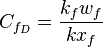 - dimensionless fracture conductivity [2],
 - proppant number [2],
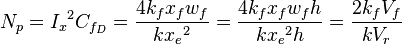
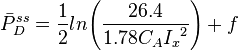
 - pseudo-steady state equation for finite-conductivity fractured wells [1],
 - steady state equation for finite-conductivity fractured wells [1],
 - shape factor [1].
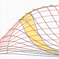
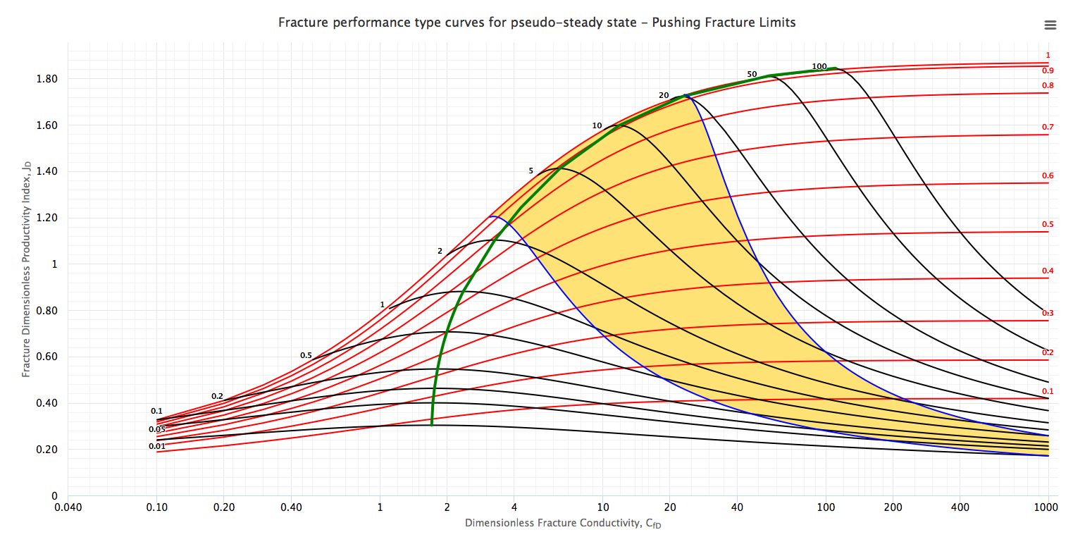
Fracturing Design Optimization Type Curves
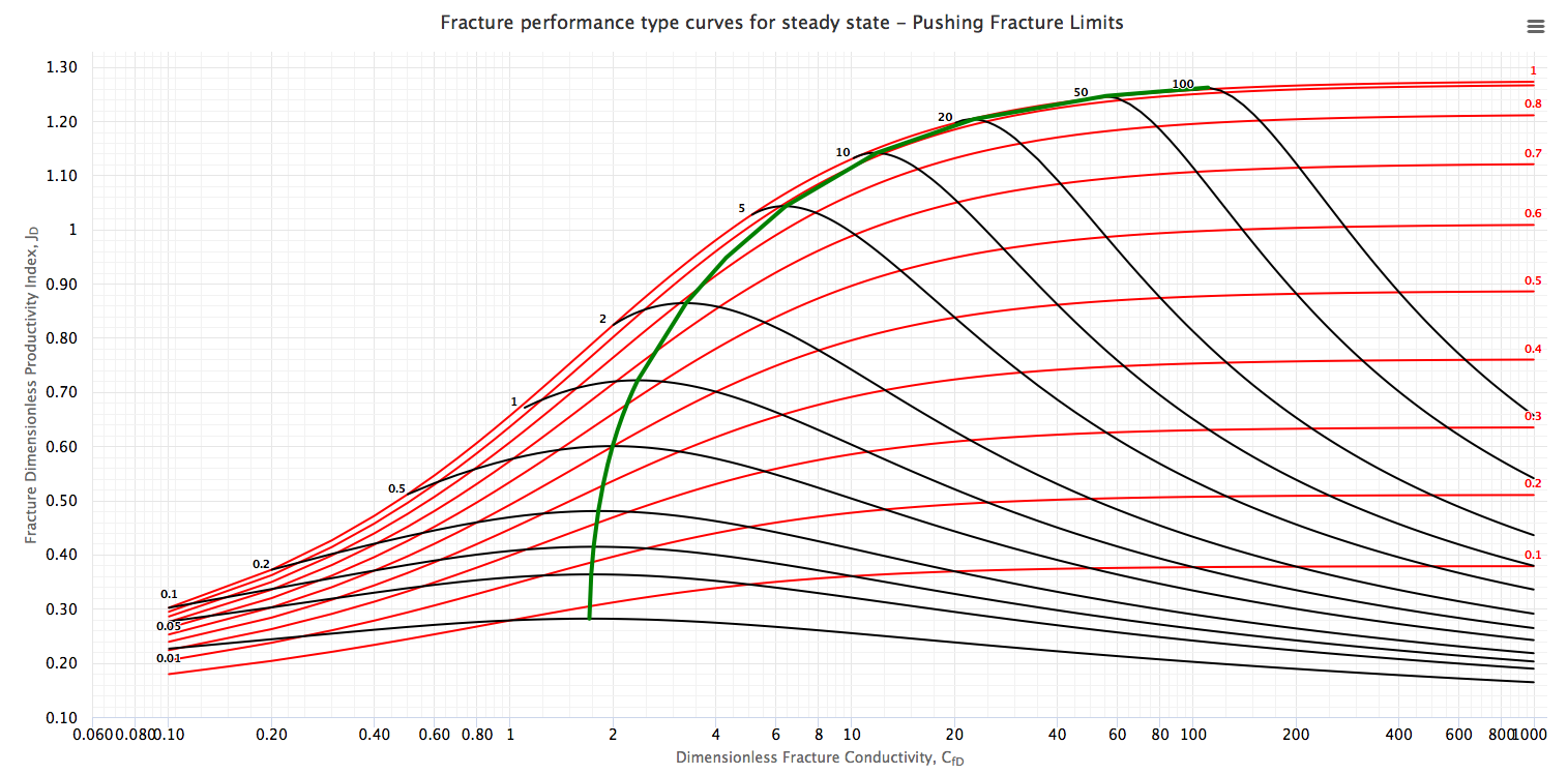
The Type Curves show the dimensionless productivity index, JD, at steady and pseudo-steady state as a function of CfD, using Ix as parameter (red curves) and overlapping with the type curve with Np as parameter (black curves).
The green curve along the maximum points for different Np values is “Design Optimization Curve”[1]. This curve represents the target of the designs of the fracture treatments in a dimensionless form.
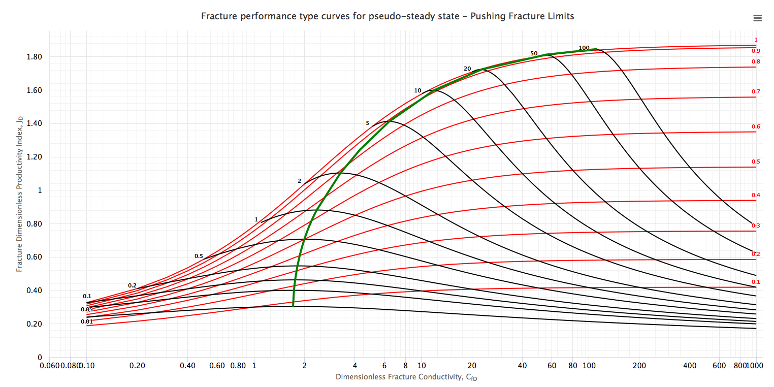
Type Curves were obtained, through seven hundred runs with a numerical simulator, modeling a fractured well in a closed square reservoir [1]. For infinite and finite fracture conductivities, the shape factors, CA, can be calculated if the PD is known for a specific value of Ix. The PD value obtained by numerical simulations. After knowing CA (which would be a function of Ix), f-function values can be calculated if PD is known for a specific dimensionless fracture conductivity CfD and fracture penetration Ix.
Fracturing Optimization Flow Diagram

Fracturing Optimization Workflow

1. Calculate the Np:
 the volume of the reservoir
 the fracture permeability
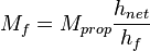 the proppant mass in the pay zone
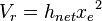
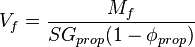 the fracture volume in the pay zone
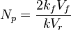 the proppant number
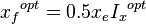
2. Read CfDopt, Ixopt, JDopt from the Design Optimization Curve of the Type Curve
3. Calculate optimum fracture half-length and width:
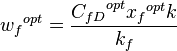
Fracturing Physical Constraints
It is important to mention that the Design Optimization Curve could give unrealistic fracture geometry depending on the reservoir permeability, reservoir mechanical properties and target Np. The two most common scenarios are [1]:
- The required net pressure for the fracture geometry is too high - “maximum net pressure curve”,
- Fracture width is too small (fracture too narrow) - “minimum width curve”.
The area between the “minimum width curve” and the “maximum net pressure curve” is the “working area” (highlighted in yellow) of the whole type curve for the specific rock mechanical properties, reservoir and proppant properties used. Any fracture design for this specific case should be located on the “optimum design curve” anywhere in this working area depending on the desired Np[1].
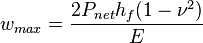
Maximum net pressure
The maximum net pressure during the fracturing treatment should provide a surface pressure less than a certain value (which is surface pressure operational limit) [1].
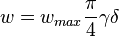
Minimum fracture width
Fracture propped width should be greater than N times mean proppant diameter (to provide at least N proppant layers in the fracture after closure)[1]. N=3 in the optiFrac.
Main features
- Fracture design Type Curves (Plot of JD as a function of CfD using Ix and Np as parameter).
- Design Optimization Curve which corresponds to the maximum JD values for different Np.
- Design Optimum Point at which JD is maximized for the given proppant, fracture and reservoir parameters.
- Physical constraints envelope.
- Hydraulic fracturing proppant catalog with predefined proppant properties.
- Users Data Worksheet for benchmarking vs actual.
- "Default values" button resets input values to the default values
- Switch between Metric and Field units
- Save/load models to the files and to the user’s cloud
- Share models to the public cloud or by using model’s link
- Export pdf report containing input parameters, calculated values and plots
- Continue your work from where you stopped: last saved model will be automatically opened
- Download the chart as an image or data and print (upper-right corner chart’s button)
- Export results table to Excel or other application
Nomenclature
 = dimensionless fracture conductivity, dimensionless
 = shape factor, dimensionless
 = Young's Modulus, psia
 = f-function, dimensionless
 = proppant permeability reduction due to gel damage, %
 = reservoir thickness, ft
 = penetration ratio, dimensionless
 = dimensionless productivity index, dimensionless
 = permeability, md
 = mass, lbm
 = dimensionless proppant number, dimensionless
 = dimensionless pressure (based on average pressure), dimensionless
 = net pressure, psia
 = specific gravity, dimensionless
 = volume, ft3
 = width, ft
 = drainage width, ft
 = fracture half-length, ft
Greek symbols
 = dry to wet width ratio at the end of pumping, usually 0.5-0.7
 = geometric factor in vertical direction, 0.75 for PKN model, 1 for KGD model
 = Poisson's ratio, dimensionless
  = porosity, fraction
 = 3.1415
Superscripts
- opt = optimal
- pss = pseudo-steady state
- ss = steady state
Subscripts
- e = external
- f = fracture
- gross = gross
- max = maximum
- net = net
- prop = proppant
- r = reservoir
References
- ↑ 1.0 1.1 1.2 1.3 1.4 1.5 1.6 1.7 1.8 1.9 Rueda, J.I.; Mach, J.; Wolcott, D. (2004). "Pushing Fracturing Limits to Maximize Producibility in Turbidite Formations in Russia"
 (SPE-91760-MS). Society of Petroleum Engineers.
- ↑ 2.0 2.1 2.2 2.3 2.4 Economides, Michael J.; Oligney, Ronald; Valko, Peter (2002). Unified Fracture Design: Bridging the Gap Between Theory and Practice. Alvin, Texas: Orsa Press.
Pages in category "OptiFrac"
The following 6 pages are in this category, out of 6 total.