Can Of Beans (Gas)

Brief

If you eat the can of beans fast then the can doesn’t last as long as if you eat it slow, but you still eat the same amount of beans.

A case study on how to increase the gas recovery factor by increasing the gas production rates.

Have you ever heard that if you increase the choke size on a gas well, the well will "die" soon, because of the water? And gas recovery will go down too?

What if you could increase the gas production and recover more gas instead?

This case study clearly demonstrates that gas recovery is increased with increasing the gas rate.

It is shown that enhanced well will add more reserves then non-enhanced well.

Case study is done using the simulation model assuring physics is well governed.

Can of beans analogy

If you eat the can of beans fast then the can doesn’t last as long as if you eat it slow, but you still eat the same amount of beans.

Same is true for the gas reservoir with bottom water.

There is a fixed volume of gas above the water.  When you remove the gas the water moves up. You can do it slow or fast but the volume of gas above the water is the same. The water level will raise Gravity stable as defined by Newton’s Law.

Simulation Runs

Now let's attach the infinite aquifer to the can of gas and run scenarios:

1. Slow - choked gas rate
2. Fast - 2x enhanced gas rate

Oh no, water killed the well quick in fast case! We told you what! Right, but … which case produced more gas?

Math and Physics

Well Nodal Analysis is done on a pressure vs rate plot. IPR and VLP curves intersect at well operating point.

Well IPR curve: Darcy's law, Vogel's IPR, Composite IPR.

Well VLP curve: Hagedorn and Brown multiphase flow correlation

Well Nodal Analysis Example

Given data:

SGg=0.65, SGo=35 API, Pr=2200 psi, Pb=1800 psi, Tr=140 F, depth = 5000ft, tubing size = 2 3/8 in OD, GOR=400 scf/stb, WOR=0
Productivity index J = 1 bbl/d/psi

It's required to find the well flowing rate at the wellhead pressure of 230 psi. Surface flow line and separator are not in question.

Solution at bottom of well

In order to solve for the flow rate at bottomhole (node position 6), the entire system is divided into two components, the reservoir or well capability component, IPR and the piping system component, VLP .

First, Vogel's equation is used to calculate the IPR curve. The AOF = 1400 bbl/d

Rate, bbl/d	Pwf, psi
0	2200
200	2000
400	1800
600	1590
800	1350
1000	1067
1400	0

Second, Hagedorn and Brown multiphase flow correlation is used to calculate the required tubing intake pressures at the given wellhead pressure, VLP curve.

Rate, bbl/d	Pwf, psi
0	1929
200	1065
400	1125
600	1181
800	1235
1000	1289
1400	1399

Third, IPR and VLP curves are plotted on the pressure vs rate plot. The intersection of these two curves shows the flow rate to be 872 bbl/d.

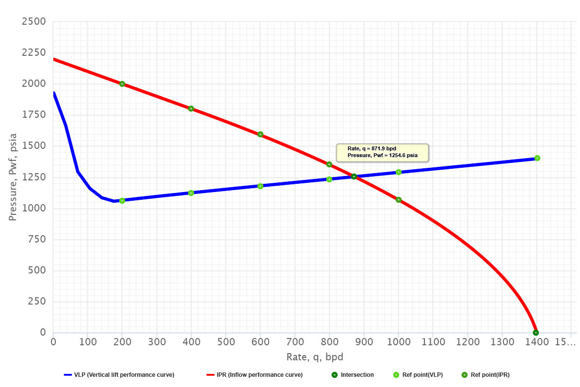
This is "the rate" possible for this system. It is not a maximum, minimum, or optimum but is the rate at which this well will produce for the piping system installed. The rate can be changed only by changing something in the system - that is, pipe sizes, choke or by shifting the IPR curve through simulation treatment.

— Kermit Brown et al

See also

• Petroleum Engineering
• Hydraulic fracturing

References

- ↑
Mach, Joe; Proano, Eduardo; Brown, Kermit E. (1979). "A Nodal Approach For Applying Systems Analysis To The Flowing And Artificial Lift Oil Or Gas Well"
(SPE-8025-MS). Society of Petroleum Engineers.
- ↑ 2.0 2.1 Brown, Kermit (1984). The Technology of Artificial Lift Methods. Volume 4. Production Optimization of Oil and Gas Wells by Nodal System Analysis. Tulsa, Oklahoma: PennWellBookss.
Cite error: <ref> tag with name "Legends" defined in <references> is not used in prior text.