Difference between revisions of "6/π stimulated well potential"
From wiki.pengtools.com
(→Math & Physics) |
(→Math & Physics) |
||
| Line 22: | Line 22: | ||
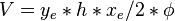
:<math> V =y_e*h*x_e/2*\phi</math> | :<math> V =y_e*h*x_e/2*\phi</math> | ||
| − | :<math>c= | + | :<math>c=\frac{1}{V} \frac{dV}{dP}</math> |
| − | :<math> \frac{dP}{dt} = | + | :<math> \frac{dP}{dt} = \frac{q}{2 c y_e h \phi} \frac{2}{x_e}</math> ( 2 ) |
( 2 ) - > ( 1 ) : | ( 2 ) - > ( 1 ) : | ||
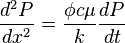
| − | :<math>\frac{d^2P}{dx^2}= | + | :<math>\frac{d^2P}{dx^2}=\frac{q \mu}{2 k y_e h} \frac{2}{x_e}</math> ( 3 ) |
Integrating ( 3 ): | Integrating ( 3 ): | ||
| − | :<math>\frac{dP}{dx}= | + | :<math>\frac{dP}{dx}=\frac{q \mu}{2 k y_e h} \frac{2}{x_e} x + c_1</math> ( 3 ) |
:<math>c_1</math> must satisfy boundary condition: | :<math>c_1</math> must satisfy boundary condition: | ||
| Line 38: | Line 38: | ||
:<math>c_1 = \frac{q \mu}{2 k y_e h}</math> | :<math>c_1 = \frac{q \mu}{2 k y_e h}</math> | ||
| − | :<math>\frac{dP}{dx}= | + | :<math>\frac{dP}{dx}=\frac{q \mu}{k x_e y_e h} \left ( x- \frac{x_e}{2} \right )</math> ( 4 ) |
Integrating ( 4 ): | Integrating ( 4 ): | ||
| − | :<math>P - P_{wf} = | + | :<math>P - P_{wf} = \frac{q \mu}{k x_e y_e h} \left ( \frac{x^2}{2} - \frac{x x_e}{2} \right )</math> ( 5 ) |
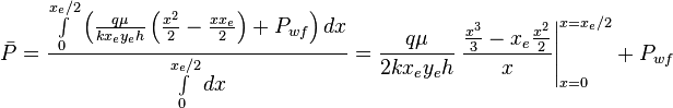
Since average pressure is: <math>\bar P = \frac{\int P dx}{\int dx}</math>: | Since average pressure is: <math>\bar P = \frac{\int P dx}{\int dx}</math>: | ||
| − | :<math> \bar P = \frac{ \int \limits_{0}^{x_e/2} \left ( | + | :<math> \bar P = \frac{ \int \limits_{0}^{x_e/2} \left ( \frac{q \mu}{k x_e y_e h} \left ( \frac{x^2}{2} - \frac{x x_e}{2} \right ) + P_{wf} \right ) dx}{\int \limits_{0}^{x_e/2}dx} = \frac{q \mu}{2 k x_e y_e h} \left. \frac{\frac{x^3}{3} - x_e \frac{x^2}{2}}{x} \right|_{x=0}^{x=x_e/2} + P_{wf} </math> |
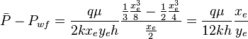
| − | :<math> \bar P - P_{wf} = | + | :<math> \bar P - P_{wf} = \frac{q \mu}{2 k x_e y_e h} \frac{\frac{1}{3} \frac{x_e^3}{8} -\frac{1}{2} \frac{x_e^3}{4}}{\frac{x_e}{2}} = \frac{q \mu}{12 k h} \frac{x_e}{y_e}</math> |
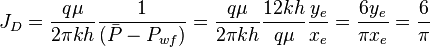
:<math>J_D=\frac{q \mu}{2 \pi k h} \frac{1}{( \bar P - P_{wf})} =\frac{q \mu}{2 \pi k h} \frac{12 k h}{q \mu} \frac{y_e}{x_e} = \frac{6 y_e}{\pi x_e}=\frac{6}{\pi}</math> | :<math>J_D=\frac{q \mu}{2 \pi k h} \frac{1}{( \bar P - P_{wf})} =\frac{q \mu}{2 \pi k h} \frac{12 k h}{q \mu} \frac{y_e}{x_e} = \frac{6 y_e}{\pi x_e}=\frac{6}{\pi}</math> | ||
Revision as of 10:25, 12 September 2018
Brief

6/π is the maximum possible stimulation potential for pseudo steady state linear flow in a square well spacing.
Math & Physics
Pseudo steady state flow boundary conditions:

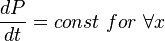
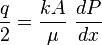
From Diffusivity Equation:
 ( 1 )
( 1 )
From Material Balance:


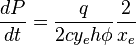 ( 2 )
( 2 )
( 2 ) - > ( 1 ) :
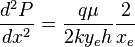 ( 3 )
( 3 )
Integrating ( 3 ):
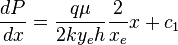 ( 3 )
( 3 )
 must satisfy boundary condition:

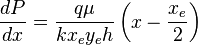 ( 4 )
( 4 )
Integrating ( 4 ):
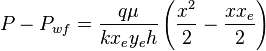 ( 5 )
( 5 )
Since average pressure is:  :
:
Diff eq
From Mass conservation:
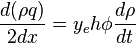 ( 1 )
( 1 )
From Darcy's law:
 ( 2 )
( 2 )

( 2 ) →( 1 ):
 ( 3 )
( 3 )
 ( 4 )
( 4 )
 ( 5 )
( 5 )
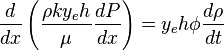
( 5 ) -> ( 4 ):
 ( 6 )
( 6 )
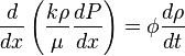
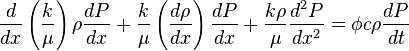 ( 7 )
( 7 )
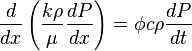
Assumption that viscosity is constant cancels out first term in left hand side of (7):
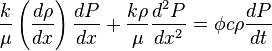 ( 8 )
( 8 )
 ( 9 )
( 9 )
( 9 ) -> ( 8 ):
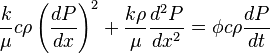 ( 10 )
Term  in (10) is second order of magnitude low and can be cancelled out, which yields:
- ( 11 )
See also
optiFrac
fracDesign
Production Potential
Nomenclature
 = cross-sectional area, cm2
 = thickness, m
 = permeability, d
 = pressure, atm
 = initial pressure, atm
 = average pressure, atm
 = flow rate, cm3/sec
 = length, m
 = drinage area length, m
 = drinage area width, m
Greek symbols
 = oil viscosity, cp