Difference between revisions of "Vogel's IPR"
(→Vogel's IPR calculation example) |
(→See also) |
||
| (19 intermediate revisions by the same user not shown) | |||
| Line 1: | Line 1: | ||
__TOC__ | __TOC__ | ||
| + | <div style='text-align: right;'>By Mikhail Tuzovskiy on {{REVISIONTIMESTAMP}}</div> | ||
==Vogel's Inflow Performance Relationship== | ==Vogel's Inflow Performance Relationship== | ||
[[File:Vogel's.png|thumb|right|300px| Vogel's IPR<ref name=Vogel />]] | [[File:Vogel's.png|thumb|right|300px| Vogel's IPR<ref name=Vogel />]] | ||
| Line 24: | Line 25: | ||
:<math> q_o = q_{ob} + (q_{o_{max}} - q_{ob}) \left (1-0.2 \frac{P_{wf}}{\bar{P}} - 0.8 \left ( \frac{P_{wf}}{\bar{P}} \right )^2 \right )</math><ref name=KermitBrown1984 /> , oil rate at given flowing bottomhole pressure. | :<math> q_o = q_{ob} + (q_{o_{max}} - q_{ob}) \left (1-0.2 \frac{P_{wf}}{\bar{P}} - 0.8 \left ( \frac{P_{wf}}{\bar{P}} \right )^2 \right )</math><ref name=KermitBrown1984 /> , oil rate at given flowing bottomhole pressure. | ||
| − | :<math> J = \frac{q_o}{\bar{P}-P_b + \frac{ | + | :<math> J = \frac{q_o}{\bar{P}-P_b + \frac{P_b}{1.8} \left (1-0.2 \frac{P_{wf}}{\bar{P}} - 0.8 \left ( \frac{P_{wf}}{\bar{P}} \right )^2 \right ) } </math><ref name=KermitBrown1984 /> , productivity index for test below the bubble point pressure. |
==Discussion == | ==Discussion == | ||
| Line 38: | Line 39: | ||
::<math>J=\frac{q_{o_{test}}}{\bar{P}-P_{wf}}</math> | ::<math>J=\frac{q_{o_{test}}}{\bar{P}-P_{wf}}</math> | ||
::* Test is below the bubble point: | ::* Test is below the bubble point: | ||
| − | ::<math> J = \frac{q_{o_{test}}}{\bar{P}-P_b + \frac{ | + | ::<math> J = \frac{q_{o_{test}}}{\bar{P}-P_b + \frac{P_b}{1.8} \left (1-0.2 \frac{P_{wf}}{\bar{P}} - 0.8 \left ( \frac{P_{wf}}{\bar{P}} \right )^2 \right ) }</math> |
:1.2 J from kh and [[JD]]: | :1.2 J from kh and [[JD]]: | ||
:: <math>J = \frac{kh\ J_D}{141.2 B \mu}</math> | :: <math>J = \frac{kh\ J_D}{141.2 B \mu}</math> | ||
:1.3 J from kh and skin: | :1.3 J from kh and skin: | ||
| − | :: <math>J = \frac{kh\ \frac{1}{1 / 0.13 + | + | :: <math>J = \frac{kh\ \frac{1}{1 / 0.13 + S}}{141.2 B \mu}</math> |
===2. Calculate the flowing rates, q<sub>o</sub>:=== | ===2. Calculate the flowing rates, q<sub>o</sub>:=== | ||
| Line 54: | Line 55: | ||
==[[Vogel's IPR]] calculation example== | ==[[Vogel's IPR]] calculation example== | ||
| − | [[File:Vogel's IPR calculation example.png|thumb|right|400px| Figure.1 Vogel's IPR calculation example]] | + | [[File:Vogel's IPR calculation example.png|thumb|right|400px| Figure.1 [https://www.pengtools.com/pqPlot?paramsToken=e9d7a7fc72e7264858153a4a9099bcf7 Vogel's IPR calculation example]]] |
Following the example problem #6, page 15 <ref name=KermitBrown1984 />: | Following the example problem #6, page 15 <ref name=KermitBrown1984 />: | ||
===Given:=== | ===Given:=== | ||
| Line 66: | Line 67: | ||
===Solution:=== | ===Solution:=== | ||
:(1) <math> q_{ob} = J (\bar{P} - P_b) = 2 \times (4200 - 3000) = 2400\ b/d</math> | :(1) <math> q_{ob} = J (\bar{P} - P_b) = 2 \times (4200 - 3000) = 2400\ b/d</math> | ||
| − | :(2) <math> q_{o_{max}} = q_{ob} + \frac{J P_b}{1.8} = 2400 + \frac{2 \times 3000}{1.8} = 2400 + 3333 = 5733 b/d</math> | + | :(2) <math> q_{o_{max}} = q_{ob} + \frac{J P_b}{1.8} = 2400 + \frac{2 \times 3000}{1.8} = 2400 + 3333 = 5733\ b/d</math> |
:(3 )<math> q_o = q_{ob} + (q_{o_{max}} - q_{ob}) \left (1-0.2 \frac{P_{wf}}{\bar{P}} - 0.8 \left ( \frac{P_{wf}}{\bar{P}} \right )^2 \right ) </math> | :(3 )<math> q_o = q_{ob} + (q_{o_{max}} - q_{ob}) \left (1-0.2 \frac{P_{wf}}{\bar{P}} - 0.8 \left ( \frac{P_{wf}}{\bar{P}} \right )^2 \right ) </math> | ||
::<math> q_o = 2400 + (5733 - 2400) \left (1-0.2 \frac{1500}{4200} - 0.8 \left ( \frac{1500}{4200} \right )^2 \right )</math> | ::<math> q_o = 2400 + (5733 - 2400) \left (1-0.2 \frac{1500}{4200} - 0.8 \left ( \frac{1500}{4200} \right )^2 \right )</math> | ||
| Line 74: | Line 75: | ||
With the help of the [[:Category:PQplot|PQplot]] software, other values of flowing pressure has been assumed, and the corresponding values of flow rate were determined. From these, the IPR cure was plotted ('''Fig.1'''). | With the help of the [[:Category:PQplot|PQplot]] software, other values of flowing pressure has been assumed, and the corresponding values of flow rate were determined. From these, the IPR cure was plotted ('''Fig.1'''). | ||
| − | The [[:Category:PQplot|PQplot]] model from this example is available online by the following link: [https://www.pengtools.com/ | + | The [[:Category:PQplot|PQplot]] model from this example is available online by the following link: [https://www.pengtools.com/pqPlot?paramsToken=e9d7a7fc72e7264858153a4a9099bcf7 Vogel's IPR calculation example] |
== Nomenclature == | == Nomenclature == | ||
:<math> B </math> = formation volume factor, bbl/stb | :<math> B </math> = formation volume factor, bbl/stb | ||
| + | :<math> J </math> = productivity index, stb/d/psia | ||
:<math> J_D </math> = dimensionless productivity index, dimensionless | :<math> J_D </math> = dimensionless productivity index, dimensionless | ||
:<math> kh</math> = permeability times thickness, md*ft | :<math> kh</math> = permeability times thickness, md*ft | ||
| + | :<math> P </math> = pressure, psia | ||
:<math> \bar{P} </math> = average reservoir pressure, psia | :<math> \bar{P} </math> = average reservoir pressure, psia | ||
| − | |||
| − | |||
| − | |||
:<math> q </math> = flowing rate, stb/d | :<math> q </math> = flowing rate, stb/d | ||
| − | :<math> | + | :<math> S </math> = skin factor, dimensionless |
| − | |||
===Greek symbols=== | ===Greek symbols=== | ||
| Line 92: | Line 91: | ||
:<math> \mu </math> = viscosity, cp | :<math> \mu </math> = viscosity, cp | ||
| − | === References | + | ===Subscripts=== |
| + | |||
| + | :b = at bubble point pressure<BR/> | ||
| + | :max = maximum<BR/> | ||
| + | :o = oil<BR/> | ||
| + | :test = well test<BR/> | ||
| + | :wf = well flowing bottomhole pressure<BR/> | ||
| + | |||
| + | == References == | ||
<references> | <references> | ||
<ref name=Vogel>{{cite journal | <ref name=Vogel>{{cite journal | ||
| Line 123: | Line 130: | ||
==See also== | ==See also== | ||
| − | :[[IPR]] | + | :[[IPR]] |
| − | :[[ | + | :[[Composite IPR]] |
| − | :[[Darcy's law]] | + | :[[3 Phase IPR]] |
| − | :[[JD]] | + | :[[Darcy's law]] |
| − | :[[ | + | :[[JD]] |
| + | :[[141.2 derivation]] | ||
{{#seo: | {{#seo: | ||
Latest revision as of 15:03, 7 April 2025
Contents
Vogel's Inflow Performance Relationship

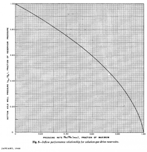
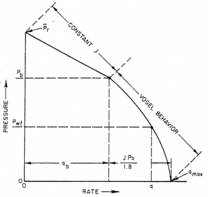
Vogel's IPR is an empirical two-phase (oil + gas) inflow performance relationship correlation published in 1968 [1].
Vogel's IPR is based on computer simulations to several solution gas drive reservoirs for different fluid and reservoir relative permeability properties.
Vogel's IPR is the default IPR correlation to calculate oil wells performance in the PQplot nodal analysis software which is available online at petroleum engineering site www.pengtools.com.
Math and Physics
Vogel's IPR equation
Darcy's law + Vogel's IPR
Combination single phase liquid constant PI equation and Vogel's IPR:
 [2] , oil flow rate at the bubble point.
 [3] , maximum oil rate or absolute open flow (AOF).
 [2] , oil rate at given flowing bottomhole pressure.
 [2] , productivity index for test below the bubble point pressure.
Discussion
Why Vogel's IPR?
Vogel's IPR solution has been found to be very good and is widely used in prediction of IPR curves.— Kermit Brown et al[2]
Vogel's IPR calculation workflow
1. Calculate the Productivity Index, J:
- 1.1 J from the flow test:
- Test is above the bubble point:

- Test is below the bubble point:

- 1.2 J from kh and JD:
-
- 1.3 J from kh and skin:
-
2. Calculate the flowing rates, qo:
For each Pwf from  to 0:
to 0:
- 2.1 Calculate oil flow rate at the bubble point:
- 2.2 Calculate maximum oil rate:
- 2.3 Calculate oil rate at given flowing bottomhole pressure, Pwf:
Vogel's IPR calculation example

Following the example problem #6, page 15 [2]:
Given:
 =4200 psi
- J=2 b/d/psi
- Pb=3000 psi
Calculate:
- (1) qob
- (2) qmax
- (3) q for Pwf=1500 psi
Solution:
- (1)

- (2)

- (3 )

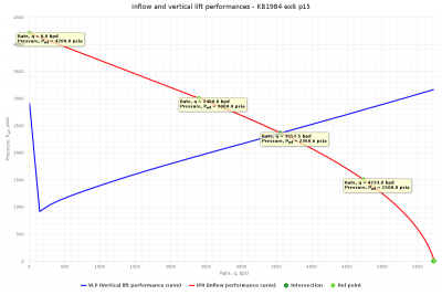
With the help of the PQplot software, other values of flowing pressure has been assumed, and the corresponding values of flow rate were determined. From these, the IPR cure was plotted (Fig.1).
The PQplot model from this example is available online by the following link: Vogel's IPR calculation example
Nomenclature
 = formation volume factor, bbl/stb
 = productivity index, stb/d/psia
 = dimensionless productivity index, dimensionless
 = permeability times thickness, md*ft
 = pressure, psia
 = average reservoir pressure, psia
 = flowing rate, stb/d
 = skin factor, dimensionless
Greek symbols
 = viscosity, cp
Subscripts
- b = at bubble point pressure
- max = maximum
- o = oil
- test = well test
- wf = well flowing bottomhole pressure
References
- ↑ 1.0 1.1 1.2 Vogel, J. V. (1968). "Inflow Performance Relationships for Solution-Gas Drive Wells". Journal of Petroleum Technology. 20 (SPE-1476-PA).
- ↑ 2.0 2.1 2.2 2.3 2.4 2.5 Brown, Kermit (1984). The Technology of Artificial Lift Methods. Volume 4. Production Optimization of Oil and Gas Wells by Nodal System Analysis. Tulsa, Oklahoma: PennWellBookss.
- ↑ Neely, A.B. (1976). Use of IPR Curves. Houston, Texas: Shell Oil Co.


