Difference between revisions of "Reservoir simulator benchmark tests"
(→Can of beans analogy) |
(→Simulation Runs) |
||
| (7 intermediate revisions by the same user not shown) | |||
| Line 1: | Line 1: | ||
==Brief == | ==Brief == | ||
| − | Before running any 3D reservoir simulator for a full scale field history matching or forecasts it is a good practice to make sure that simulator is performing well on a simple benchmark tests with well known analytical solutions. | + | Before running any 3D reservoir simulator for a full scale field history matching or forecasts it is a good practice to make sure that the simulator is performing well on a simple benchmark tests with the well known analytical solutions. |
| − | + | By running those cases you could get ahead of the learning curve and gain confidence in your simulation results. | |
| − | |||
| − | + | ==Calculating well potential== | |
| − | + | Analytical equations are available to calculate the flow rate potential for unstimulated and stimulated wells. | |
| + | Steady state and pseudo steady state flow regimes are considered. | ||
| − | ==Simulation Runs== | + | ===Simulation Test Runs=== |
| − | + | #Vertical well in a square drainage area pseudo steady state flow | |
| − | # | + | #Vertical well in a square drainage area steady state flow |
| − | # | + | #Fracture vertical well in a square drainage area pseudo steady state flow |
| − | + | #Fractured vertical well in a square drainage area steady state flow | |
| − | + | #Horizontal well in a square drainage area pseudo steady state flow | |
| − | + | #Horizontal well in a square drainage area steady state flow | |
| − | + | #Horizontal well with orthogonal fractures in a rectangular drainage area pseudo steady state flow | |
| + | #Horizontal well with orthogonal fractures in a rectangular drainage area steady state flow | ||
==Gas Recovery== | ==Gas Recovery== | ||
| Line 72: | Line 73: | ||
*qgas_slow = 100 000 m3/d | *qgas_slow = 100 000 m3/d | ||
*qgas_fast = 200 000 m3/d | *qgas_fast = 200 000 m3/d | ||
| + | |||
| + | ===3D reservoir simulation software=== | ||
| + | *ECLIPSE | ||
| + | *tNavigator | ||
| + | *CMG | ||
| + | *Waiwera | ||
== See also == | == See also == | ||
Latest revision as of 17:27, 7 August 2023
Contents
Brief
Before running any 3D reservoir simulator for a full scale field history matching or forecasts it is a good practice to make sure that the simulator is performing well on a simple benchmark tests with the well known analytical solutions.
By running those cases you could get ahead of the learning curve and gain confidence in your simulation results.
Calculating well potential
Analytical equations are available to calculate the flow rate potential for unstimulated and stimulated wells. Steady state and pseudo steady state flow regimes are considered.
Simulation Test Runs
- Vertical well in a square drainage area pseudo steady state flow
- Vertical well in a square drainage area steady state flow
- Fracture vertical well in a square drainage area pseudo steady state flow
- Fractured vertical well in a square drainage area steady state flow
- Horizontal well in a square drainage area pseudo steady state flow
- Horizontal well in a square drainage area steady state flow
- Horizontal well with orthogonal fractures in a rectangular drainage area pseudo steady state flow
- Horizontal well with orthogonal fractures in a rectangular drainage area steady state flow
Gas Recovery
_recovery.png)
12% more recovery with the enhanced production over 20 years. Why?
Because of the pressure! The lower the reservoir pressure the more gas is produced before the water hits the perfs. It’s just physics!
_pressure.png)
Math and Physics
According to the Boyle's law (1662):
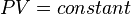
where P is pressure, V is volume.
In our case

The gas produced volume of the "Slow case"

The gas produced volume of the "Fast case"
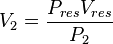
And V2 > V1 because P2 < P1. The lower the P2 gets over P1 the higher the incremental recovery will be.
Summary
Produce gas reservoirs fast to increases recoveries.
If you have an aquifer you have to produce fast.
If you don’t have an aquifer…, so you don’t have water to complain.
Video
Watch our video explaining the gas reservoir production using the Can Of Beans (Gas) as an example
_video.png)
Model overview
_model.png)
- Cylindrical grid (10x10x30)
- re=500m, rw=0.1m, h=30m
- kx=ky=5mD, kz/kx=0.1, phi=0.2
- Pi=300bar, hres=3000m
- Gas and water PVT model
- SGgas=0.58
- Aquifer at the bottom (CT infinite extent)
- qgas_slow = 100 000 m3/d
- qgas_fast = 200 000 m3/d
3D reservoir simulation software
- ECLIPSE
- tNavigator
- CMG
- Waiwera
See also
References
Cite error: <ref> tag defined in <references> has group attribute "" which does not appear in prior text.