Gray correlation
From wiki.pengtools.com
Contents
Brief
Gray is an empirical two-phase flow correlation published in 1974 [1].
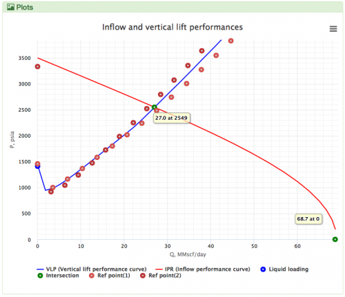
Gray is the default VLP correlation for the gas wells in the PQplot.
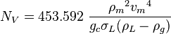
Math & Physics
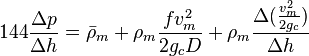
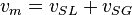
Following the law of conservation of energy the basic steady state flow equation is:
where
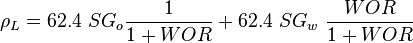
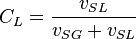
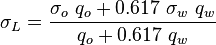
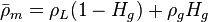 , slip mixture density [1].
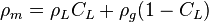 , no-slip mixture density [1].
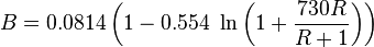
Colebrook–White [2] equation for the Darcy's friction factor:
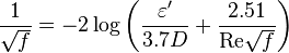
The pseudo wall roughness:
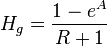
 , with the limit
 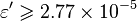 [1]
[1]
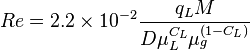
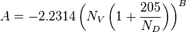
Reynolds two phase number:
Discussion
Why Gray correlation?
The Gray correlation was found to be the best of several initially tested ...— Nitesh Kumar l[5]
Workflow Hg & CL


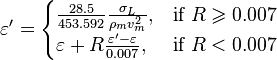
Modifications
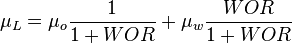
1. Use Fanning correlation for the dry gas (WGR=0 and OGR=0 case).
2. Use watercut instead of WOR to account for the OGR=0 case.
3. If the relative roughness:  use 0.05 in the Moody Diagram [3].
4. If HL can't be calculated then HL = CL.
Nomenclature
 = correlation group, dimensionless
 = flow area, ft2
 = correlation group, dimensionless
- = formation factor, bbl/stb
 = no-slip holdup factor, dimensionless
 = pipe diameter, ft
 = depth, ft
 = holdup factor, dimensionless
 = friction factor, dimensionless
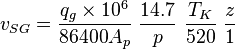
 = gas-liquid ratio, scf/bbl
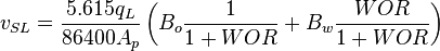
 = total mass of oil, water and gas associated with 1 bbl of liquid flowing into and out of the flow string, lbm/bbl
 = pipe diameter number, dimensionless
 = velocity number, dimensionless
 = pressure, psia
 = conversion constant equal to 32.174049, lbmft / lbfsec2
 = production rate, bbl/d
 = superficial liquid to gas ratio, dimensionless
 = Reynolds number, dimensionless
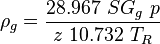
 = specific gravity, dimensionless
 = temperature, °R or °K, follow the subscript
 = velocity, ft/sec
 = water-oil ratio, bbl/bbl
 = gas compressibility factor, dimensionless
Greek symbols
 = absolute roughness, ft
 = pseudo wall roughness, ft
 = viscosity, cp
 = density, lbm/ft3
 = slip density, lbm/ft2
 = surface tension of liquid-air interface, dynes/cm
Subscripts
g = gas
K = °K
L = liquid
m = gas/liquid mixture
o = oil
R = °R
SL = superficial liquid
SG = superficial gas
w = water
References
- ↑ 1.00 1.01 1.02 1.03 1.04 1.05 1.06 1.07 1.08 1.09 1.10 Gray, H. E. (1974). "Vertical Flow Correlation in Gas Wells". User manual for API 14B, Subsurface controlled safety valve sizing computer program. API.
- ↑ Colebrook, C. F. (1938–1939). "Turbulent Flow in Pipes, With Particular Reference to the Transition Region Between the Smooth and Rough Pipe Laws"
 . Journal of the Institution of Civil Engineers. London, England. 11: 133–156.
- ↑ 3.0 3.1 Moody, L. F. (1944). "Friction factors for pipe flow". Transactions of the ASME. 66 (8): 671–684.
- ↑ 4.0 4.1 Hagedorn, A. R.; Brown, K. E. (1965). "Experimental study of pressure gradients occurring during continuous two-phase flow in small-diameter vertical conduits". Journal of Petroleum Technology. 17(04): 475–484.
- ↑ Kumar, N.; Lea, J. F. (January 1, 2005). "Improvements for Flow Correlations for Gas Wells Experiencing Liquid Loading"
 (SPE-92049-MS).
- ↑ 6.0 6.1 6.2 Lyons, W.C. (1996). Standard handbook of petroleum and natural gas engineering. 2. Houston, TX: Gulf Professional Publishing. ISBN 0-88415-643-5.