Difference between revisions of "Gas Flowing Material Balance"

Revision as of 12:28, 11 December 2017

Brief

Gas Flowing Material Balance is the advanced engineering technique to determine the Reservoirs GIIP and recovery as well as Well's EUR and JD.

Gas Flowing Material Balance is applied on the Well level given readily available well flowing data: production rate and tubing head pressure.

The interpretation technique is fitting the data points with the straight line to estimate GIIP and JD.

Math & Physics

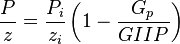
Combining the gas pseudo state flow equation and the Gas Material Balance equation to get Gas Flowing Material Balance equation:

P_{\bar{P}}= P_{P_{wf}} + q_g b_{pss}

^[1]

where

b_{pss} = \frac{1422 \times 10^3\ T_R}{kh\ J_D}

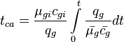
Material balance pseudo-time:

t_{ca} = \frac{\mu_{gi} c_{gi}}{q_g}\int\limits_{0}^{t}\frac{q_g}{\bar{\mu_g} \bar{c_g}}dt

Discussion

well vs reservoir model start

Workflow

Calculate the red line:
1. Given the GIIP
2. Calculate the $\frac{P}{z}=\frac{P_i}{z_i} \left (1- \frac{G_p}{GIIP}\right )$
Calculate the orange curve:
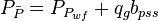
1. Given the flowing wellhead pressures, calculate the flowing bottomhole pressures, $P_{wf}$
2. Convert the flowing pressures to pseudopressures, $P_{P_{wf}}$
3. Given the JD, calculate the $b_{pss}$
4. Calculate the pseudopressure, $P_{\bar{P}}$
5. Convert the pseudopressure to pressure, $\bar{P}$
6. Calculate the $\frac{\bar{P}}{z}$
Calculate the gray JD curve:
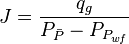
1. Calculate the gas productivity index, $J=\frac{q_g}{P_{\bar{P}}-P_{P_{wf}}}$
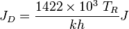
2. Calculate the JD, $J_D=\frac{1422 \times 10^3\ T_R}{kh} J$
Change the red line to match the orange curve
1. Change the GIIP
2. Change the intitial $\frac{P}{z}$
Change the flat JD gray line to match the changing JD gray line
Save the Gas Flowing Material Balance model
Move to the next well

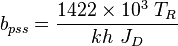
Extra Plot to find b_pss

Calculate the initial pseudopressure, $P_{Pi}$
Calculate the material balance pseudo-time, $t_{ca}$
Plot $\frac{P_{P_i}-P_{P_{wf}}}{q_g}$ versus $t_{ca}$
The intercept with the Y axis gives $b_{pss}$ and $J_D$

Data required

Create Field here
Upload Wells here
Upload Daily Measures here
Create or Upload Reservoirs here
Input the Reservoirs GIIP here
Create or Upload PVT (SG, Pi, Ti) here
Create or Upload Wells Perforations here
Create or Upload kh and JD here
Create or Upload the static reservoir pressures, here
Export static reservoir pressures to Daily Measures here
Calculate the flowing bottomhole pressures using BHP Calculator
Export flowing bottomhole pressures to Daily Measures here

Nomenclature

b_{pss}

= reservoir constant, inverse to productivity index, psia²/cP/MMscfd

c

= compressibility, psia^-1

GIIP

= gas initially in place, MMscf

G_p

= cumulative gas produced, MMscf

J

= gas productivity index, MMscfd/(psia²/cP)

J_D

= dimensionless productivity index, dimensionless

kh

= permeability times thickness, md*m

P

= pressure, psia

\bar{P}

= average reservoir pressure, psia

P_P

= pseudopressure, psia²/cP

q_g

= gas rate, MMscfd

t

= time, day

t_{ca}

= material balance pseudotime for gas, day

T

= temperature, °R

z

= gas compressibility factor, dimensionless

Greek symbols

\mu

= viscosity, cp

Subscripts

g = gas

i = initial

R = °R

wf = well flowing

References

↑ Mattar, L.; Anderson, D (2005). "Dynamic Material Balance (Oil or Gas-In-Place Without Shut-Ins)" (PDF). CIPC.

[Mattar2005-1] Mattar, L.; Anderson, D (2005). "Dynamic Material Balance (Oil or Gas-In-Place Without Shut-Ins)" (PDF). CIPC.

[1]

@@ Line 58: / Line 58: @@
 * Upload [[Daily Measures]] [https://ep.pengtools.com/daily/measures/upload  here]
 * Create or Upload [[Reservoirs]] [https://ep.pengtools.com/reservoir/index here]
-* Input the [[Reservoirs]] GIIP
+* Input the [[Reservoirs]] GIIP [https://ep.pengtools.com/reservoir/index here]
 * Create or Upload [[PVT]] (SG, Pi, Ti) [https://ep.pengtools.com/pvt/index here]
 * Create or Upload [[Well]]s Perforations [https://ep.pengtools.com/perforation/index here]

Navigation menu

Navigation

Categories

Products

Difference between revisions of "Gas Flowing Material Balance"

Revision as of 12:28, 11 December 2017

Contents

Brief

Math & Physics

Discussion