Beggs and Brill correlation
Contents
Brief
Beggs and Brill is an empirical two-phase flow correlation published in 1972 [1].
It distinguish between 4 flow regimes.
Beggs and Brill is the default VLP correlation in sPipe.
Math & Physics
Fluid flow energy balance
where
Flow patterns
Froude number:
SEGREGATED:  [2]
[2]
TRANSITION:  [2]
[2]
INTERMITTENT:  [2]
[2]
DISTRIBUTED:  [2]
[2]
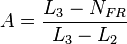
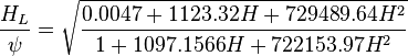
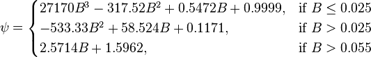
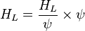
Liquid Holdup HL
SEGREGATED, INTERMITTENT, DISTRIBUTED: 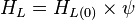 [2]
[2]
TRANSITION:  [2]
[2]
where:
Friction factor
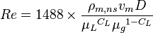
No slip Reynolds two phase number:
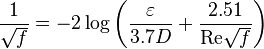
Colebrook–White [3] equation for the Darcy's friction factor:
Corrected two phase friction factor:

where

and

with constraint:

Discussion
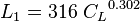
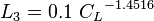
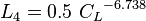
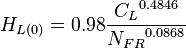
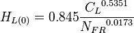
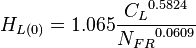
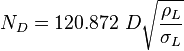
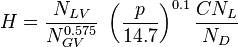
Why Hagedorn and Brown?
One of the consistently best correlations ...— Michael Economides et al[5]
Flow Diagram

Workflow


Determine the flow pattern: SEGREGATED, INTERMITTENT, DISTRIBUTED, TRANSITION.

with the constraint  [2]
[2]
C Uphill:


C Downhill:
- ALL:
 [2]
[2]

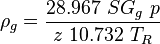
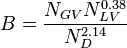
![N_L = 0.15726\ \mu_L \sqrt[4]{\frac{1}{\rho_L \sigma_L^3}}](/images/math/b/2/0/b207fe79b4a4ee53d466e182791ca737.png)

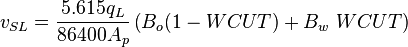
![N_{LV} = 1.938\ v_{SL}\ \sqrt[4]{\frac{\rho_L}{\sigma_L}}](/images/math/d/d/8/dd824df0b6ec22aa724161b929e993fe.png)
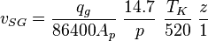
![N_{GV} = 1.938\ v_{SG}\ \sqrt[4]{\frac{\rho_L}{\sigma_L}}](/images/math/3/6/4/364153c39c1657b3b7bab8f7ed710e60.png)
Modifications
1. Use the no-slip holdup when the original empirical correlation predicts a liquid holdup HL less than the no-slip holdup [5].
2. Use the Griffith correlation to define the bubble flow regime[5] and calculate HL.
3. Use watercut instead of WOR to account for the watercut = 100%.
Nomenclature
 = flow area, ft2
 = correlation group, dimensionless
- = formation factor, bbl/stb
 = coefficient for liquid viscosity number, dimensionless
 = pipe diameter, ft
 = depth, ft
 = correlation group, dimensionless
 = liquid holdup factor, dimensionless
 = friction factor, dimensionless
 = gas-liquid ratio, scf/bbl
 = total mass of oil, water and gas associated with 1 bbl of liquid flowing into and out of the flow string, lbm/bbl
 = pipe diameter number, dimensionless
 = gas velocity number, dimensionless
 = liquid viscosity number, dimensionless
 = liquid velocity number, dimensionless
 = pressure, psia
 = conversion constant equal to 32.174049, lbmft / lbfsec2
 = total liquid production rate, bbl/d
 = Reynolds number, dimensionless
 = solution gas-oil ratio, scf/stb
 = specific gravity, dimensionless
 = temperature, °R or °K, follow the subscript
 = velocity, ft/sec
 = water-oil ratio, bbl/bbl
 = gas compressibility factor, dimensionless
Greek symbols
 = absolute roughness, ft
 = viscosity, cp
 = density, lbm/ft3
 = integrated average density at flowing conditions, lbm/ft2
 = surface tension of liquid-air interface, dynes/cm (ref. values: 72 - water, 35 - oil)
 = secondary correlation factor, dimensionless
Subscripts
g = gas
K = °K
L = liquid
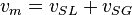
m = gas/liquid mixture
o = oil
R = °R
SL = superficial liquid
SG = superficial gas
w = water
References
- ↑ 1.0 1.1 1.2 1.3 Beggs, H. D.; Brill, J. P. (May 1973). "A Study of Two-Phase Flow in Inclined Pipes"
 . Journal of Petroleum Technology. AIME. 255 (SPE-4007-PA).
- ↑ 2.00 2.01 2.02 2.03 2.04 2.05 2.06 2.07 2.08 2.09 2.10 2.11 2.12 2.13 2.14 2.15 2.16 2.17 2.18 2.19 2.20 2.21 2.22 2.23 2.24 Cite error: Invalid
<ref>tag; no text was provided for refs namedBB1991 - ↑ Colebrook, C. F. (1938–1939). "Turbulent Flow in Pipes, With Particular Reference to the Transition Region Between the Smooth and Rough Pipe Laws". Journal of the Institution of Civil Engineers. London, England. 11: 133–156.
- ↑ Moody, L. F. (1944). "Friction factors for pipe flow". Transactions of the ASME. 66 (8): 671–684.
- ↑ 5.0 5.1 5.2 5.3 5.4 5.5 Economides, M.J.; Hill, A.D.; Economides, C.E.; Zhu, D. (2013). Petroleum Production Systems (2 ed.). Westford, Massachusetts: Prentice Hall. ISBN 978-0-13-703158-0.
- ↑ 6.0 6.1 6.2 6.3 6.4 6.5 6.6 Lyons, W.C. (1996). Standard handbook of petroleum and natural gas engineering. 2. Houston, TX: Gulf Professional Publishing. ISBN 0-88415-643-5.
- ↑ 7.0 7.1 7.2 7.3 7.4 Cite error: Invalid
<ref>tag; no text was provided for refs namedHB - ↑ 8.0 8.1 Trina, S. (2010). An integrated horizontal and vertical flow simulation with application to wax precipitation (Master of Engineering Thesis). Canada: Memorial University of Newfoundland.