Difference between revisions of "Oil Flowing Material Balance"
(→Brief) |
(→References) |
||
| Line 119: | Line 119: | ||
|date=2005 | |date=2005 | ||
|url=https://www.ihs.com/pdf/dynamic-material-balance-paper_227867110913049832.pdf | |url=https://www.ihs.com/pdf/dynamic-material-balance-paper_227867110913049832.pdf | ||
| + | }}</ref> | ||
| + | |||
| + | <ref name=Stalgorova2016>{{cite journal | ||
| + | |last1= Stalgorova |first2=Ekaterina | ||
| + | |last2=Mattar|first1=Louis | ||
| + | |title=Analytical Methods for Single-Phase Oil Flow: Accounting for Changing Liquid and Rock Properties | ||
| + | |publisher=Society of Petroleum Engineers | ||
| + | |date=2016 | ||
| + | |url=https://www.onepetro.org/conference-paper/SPE-180139-MS?sort=&start=0&q=SPE-180139-MS&from_year=&peer_reviewed=&published_between=&fromSearchResults=true&to_year=&rows=25# | ||
}}</ref> | }}</ref> | ||
Revision as of 05:57, 10 April 2018
Contents
Brief
Oil Flowing Material Balance (Oil FMB) is the advanced engineering technique published in 2005 by Louis Mattar and David Anderson [1].
Oil Flowing Material Balance is applied to determine:
- Reservoirs STOIIP & EUR
- Well's EUR and JD
Oil Flowing Material Balance uses readily available Welll flowing data: production rate and bottomhole pressure.
The interpretation technique is fitting the data points with the straight lines to estimate STOIIP and JD.
Math & Physics
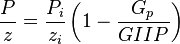
Combining the gas pseudo state flow equation and the Gas Material Balance equation to get Gas Flowing Material Balance equation:
where
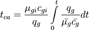
Material balance pseudo-time:
Discussion
Gas Flowing Material Balance can be applied to:
- single well
- multiple wells producing from the same Reservoir.
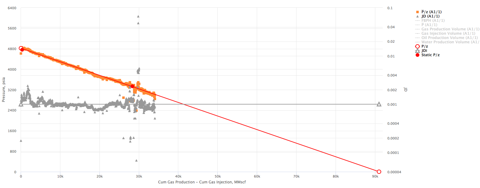
The X axis on the Gas Flowing Material Balance Plot can be selected as:
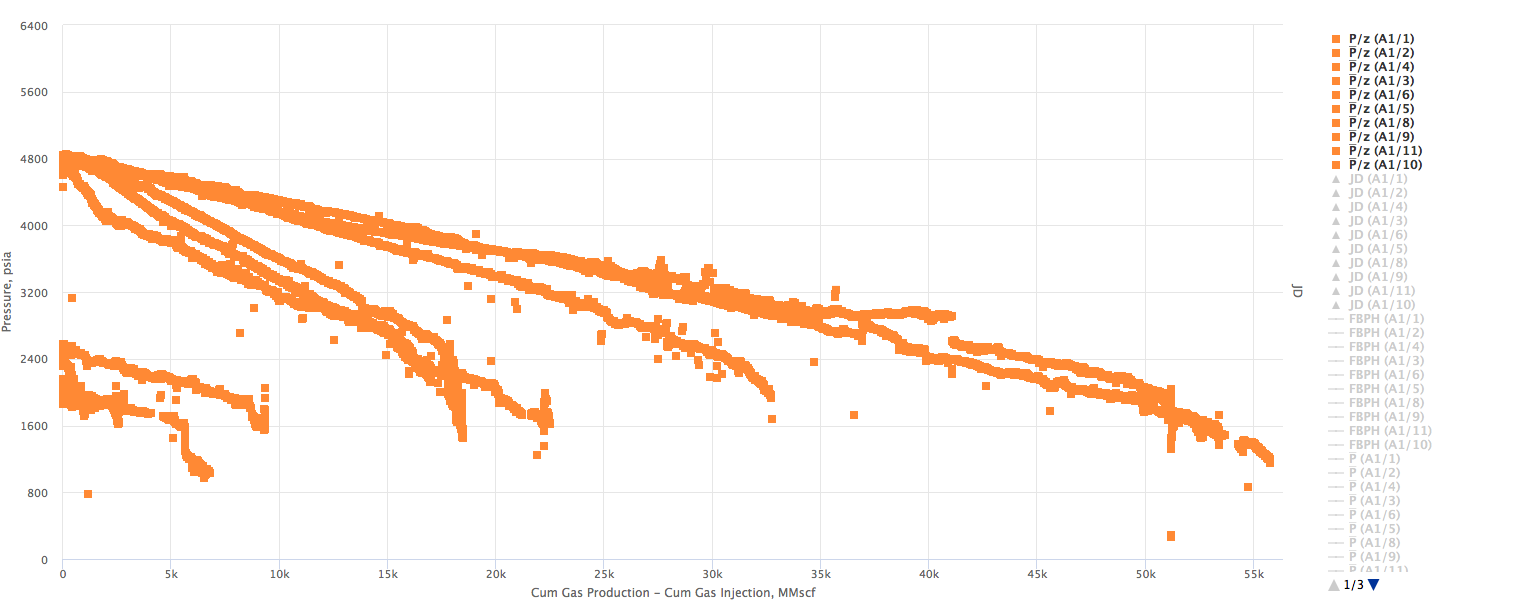
Example 1. Multiple wells producing from the same Reservoir. X axis - Wells cumulative
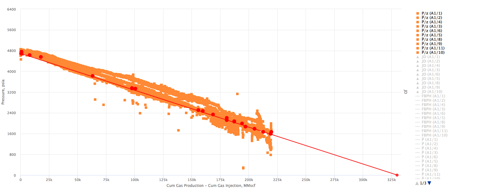
 Example 2. Multiple wells producing from the same Reservoir. X axis - Reservoir cumulative
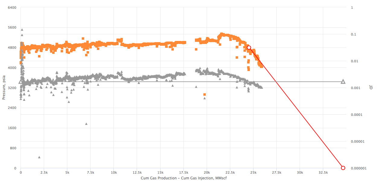
 Example 3. Shifted Model Start (to account for gas injection)
Workflow
- Upload the data required
- Open the Gas Flowing Material Balance tool here
- Calculate the red
 line:
line:
- Given the GIIP
- Calculate the
- Calculate the orange
 curve:
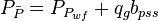
- Given the flowing wellhead pressures, calculate the flowing bottomhole pressures,

- Convert the flowing pressures to pseudopressures,

- Given the JD, calculate the

- Calculate the pseudopressure,

- Convert the pseudopressure to pressure,

- Calculate the
- Given the flowing wellhead pressures, calculate the flowing bottomhole pressures,
- Calculate the gray JD curve:
- Calculate the gas productivity index,
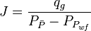
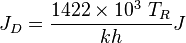
- Calculate the JD,
- Calculate the gas productivity index,
- Change the red line to match the orange curve
- Change the GIIP
- Change the intitial
- Change the flat JD gray line to match the changing JD gray line
- Save the FMB model
- Move to the next well
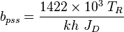
Extra Plot to find bpss
- Calculate the initial pseudopressure,

- Calculate the material balance pseudo-time,

- Plot
 versus
 - The intercept with the Y axis gives and

Data required
- Create Field here
- Create or Upload Reservoirs here
- Input the Reservoirs GIIP and STOIIP here
- Create or Upload PVT (SG, Pi, Ti) here
- Upload Wells
- Create or Upload Wells Perforations here
- Create or Upload kh and JD here
- Upload Daily Measures
In case you need to calculate the flowing bottomhole pressure from the wellhead pressure:
- Calculate the flowing bottomhole pressures using BHP Calculator
- Export flowing bottomhole pressures to Daily Measures here
In case you want to add the static reservoir pressures on the FMB Plot:
- Create or Upload the static reservoir pressures, here
- Calculate Monthly Measures from the Daily Measures using Monthly Data Calculator
Nomenclature
- = reservoir constant, inverse to productivity index, psia2/cP/MMscfd
 = compressibility, psia-1
 = gas initially in place, MMscf
 = cumulative gas produced, MMscf
 = gas productivity index, MMscfd/(psia2/cP)
- = dimensionless productivity index, dimensionless
 = permeability times thickness, md*m
 = pressure, psia
- = average reservoir pressure, psia
 = pseudopressure, psia2/cP
 = gas rate, MMscfd
 = time, day
- = material balance pseudotime for gas, day
 = temperature, °R
 = gas compressibility factor, dimensionless
Greek symbols
 = viscosity, cp
Subscripts
- g = gas
- i = initial
- R = °R
- wf = well flowing
References
- ↑ 1.0 1.1 Mattar, L.; Anderson, D (2005). "Dynamic Material Balance (Oil or Gas-In-Place Without Shut-Ins)" (PDF). CIPC.
Cite error: <ref> tag with name "Stalgorova2016" defined in <references> is not used in prior text.