Difference between revisions of "Hall Plot"
(→Hall Plot Application with Wellhead Pressure) |
(→Hall Plot Application with Wellhead Pressure) |
||
| Line 35: | Line 35: | ||
Rearranging above: | Rearranging above: | ||
| − | :<math> \sum P_{ | + | :<math> \sum P_{tub} \Delta t = \frac{141.2 B \mu}{kh J_D} \times \left( \sum q_{inj} \right) + \left( \sum \bar{P} - \sum \Delta P_{friction} - \sum \Delta P_{gravity} \right) \Delta t </math> |
| − | |||
== Nomenclature == | == Nomenclature == | ||
Revision as of 16:32, 27 August 2026
Contents
Brief
Hall Plot is the engineering technique to analyze performance of injection wells published in 1963 by Howard Hall [1].
Hall Plot is applied to determine the change in the Injectivity index of the wells.
Hall Plot uses readily available Well flowing data: injection rate and wellhead pressures.
The interpretation technique is fitting the data points with the straight lines to estimate injectivity change.
Math & Physics
From Darcy's law for an unfractured injection well located in the center of a circular drainage area, the injection rate in pseudo-steady state is:

Hall integrated both sides with respect to time [2]:

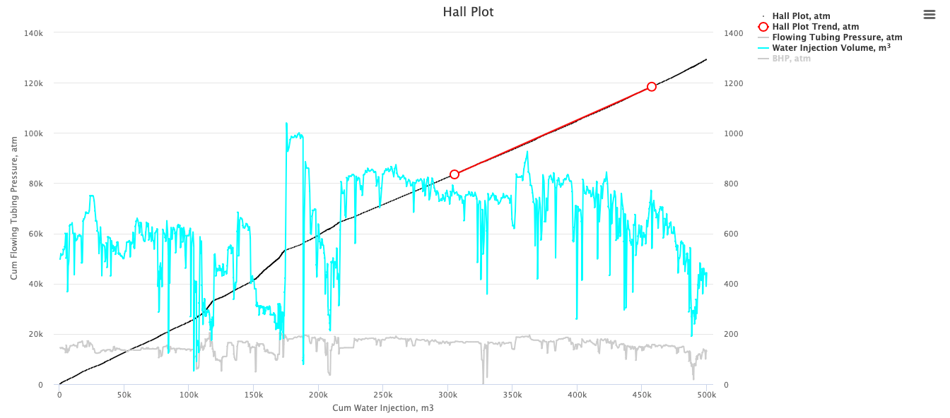
The Cartesian graph of cumulative injection versus cumulative  yields a straight line with slope:
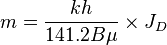
and Injectivity index is:

Hall Plot Application with Wellhead Pressure
Since bottomhole and reservoir pressures are not readily available, the Hall Plot can be used with tubing head pressure.
Given:

Rearranging above:

Nomenclature
See Also
- ↑ Hall, H.N. (1963). "How To Analyze Waterflood Injection Well Performance". World Oil.
- ↑ Buell, R.S.; Kazemi, H.; Poettmann, F.H. (1990). "Analyzing Injectivity of Polymer Solutions With the Hall Plot". SPE Reservoir Engineering. 5 (1). doi:10.2118/16963-PA.