Difference between revisions of "Hall Plot"
(→Hall Plot Application with Wellhead Pressure) |
(→Discussion) |
||
| (50 intermediate revisions by the same user not shown) | |||
| Line 8: | Line 8: | ||
The interpretation technique is fitting the data points with the straight lines to estimate injectivity change. | The interpretation technique is fitting the data points with the straight lines to estimate injectivity change. | ||
| + | |||
| + | [[Hall Plot]] is available online at [https://ep.pengtools.com/daily/measures/water-injectors E&P Portal]. | ||
| + | |||
[[File:Hall Plot.png|link=https://ep.pengtools.com/waterflooding/hall-plot]] | [[File:Hall Plot.png|link=https://ep.pengtools.com/waterflooding/hall-plot]] | ||
| − | <center>[[Hall Plot]] in the [https://ep.pengtools.com/ | + | <center>[[Hall Plot]] in the [https://ep.pengtools.com/daily/measures/water-injectors E&P Portal]</center> |
==Math & Physics== | ==Math & Physics== | ||
| Line 19: | Line 22: | ||
Hall integrated both sides with respect to time <ref name=Buell1990/>: | Hall integrated both sides with respect to time <ref name=Buell1990/>: | ||
:<math> \sum q_{inj} \Delta t = \frac{kh}{141.2 B \mu} \times J_D \times \sum (P_{wf} - \bar{P}) \Delta t </math> | :<math> \sum q_{inj} \Delta t = \frac{kh}{141.2 B \mu} \times J_D \times \sum (P_{wf} - \bar{P}) \Delta t </math> | ||
| − | The Cartesian graph of | + | The Cartesian graph of cumulative <math>(P_{wf} - \bar{P})</math> versus cumulative injection yields a straight line with slope: |
| − | :<math> m = \frac | + | :<math> m = \frac{141.2 B \mu}{khJ_D} </math> |
and [[Injectivity index]] is: | and [[Injectivity index]] is: | ||
| Line 29: | Line 32: | ||
===Hall Plot Application with Wellhead Pressure=== | ===Hall Plot Application with Wellhead Pressure=== | ||
| − | Since bottomhole | + | Since bottomhole and reservoir pressures are not readily available, the [[Hall Plot]] can be used with tubing head pressure. |
| + | |||
| + | Given: | ||
| + | :<math> P_{wf} = P_{tub} + \Delta P_{friction} + \Delta P_{gravity} </math> | ||
| − | = | + | Rearranging above: |
| + | :<math> \sum P_{tub} \Delta t = \frac{141.2 B \mu}{kh J_D} \times \sum q_{inj} \Delta t + \sum ( \bar{P} - \Delta P_{friction} - \Delta P_{gravity} ) \Delta t </math> | ||
| − | + | Under the assumption that the reservoir pressure, friction and gravity terms are constant, a plot of cumulative tubing head pressure versus cumulative injection will yield a straight line. The slope of this line represents the '''apparent injectivity''', which includes the effects of friction, gravity, and reservoir pressure. | |
| − | + | ==Discussion== | |
| − | |||
| + | The [[Hall Plot]] is primarily used for qualitative analysis of injectivity changes. A change in slope may indicate: | ||
| − | + | *Increasing slope indicates formation damage, scaling, increasing skin, or external radius decrease. | |
| − | + | *Decreasing slope indicates stimulation, fracturing, increasing water relative permeability (e.g., with surfactant), or increasing well radius (e.g., with acid). | |
| + | *Constant slope indicates constant skin, reservoir pressure, wellbore radius, external radius and permeability-thickness (kh). | ||
| + | |||
| + | Early in the life of a waterflood, the [[Hall Plot]] may exhibit a concave upward appearance. This is caused by the expansion of the external drainage radius and increase in reservoir pressure <ref name=DW/>. | ||
| + | |||
| + | The tubing head pressure plot serves as a first-step diagnostic. Any slope changes observed should be verified with a cumulative <math>P_{wf} - \bar{P}</math> versus cumulative <math>q_{inj}</math> plot for confirmation. | ||
| + | |||
| + | Multiple wells can be plotted on the same Hall Plot for comparison. This allows for easy identification of wells that are underperforming or responding to stimulation. | ||
| + | |||
| + | [[File:Multiple_wells_Hall_Plot.png|Hall Plot example for multiple wells]] | ||
| + | |||
| + | <center>[[Hall Plot]] for multiple wells in the [https://ep.pengtools.com/daily/measures/water-injectors E&P Portal]</center> | ||
== Nomenclature == | == Nomenclature == | ||
| − | == | + | :<math> B </math> = formation volume factor, bbl/stb |
| − | + | :<math> I </math> = injectivity index, stb/d/psia | |
| + | :<math> J_D </math> = dimensionless injectivity index, dimensionless | ||
| + | :<math> kh </math> = permeability times thickness, md·ft | ||
| + | :<math> m </math> = slope of Hall Plot, psia·d/bbl | ||
| + | :<math> P_{wf} </math> = bottomhole flowing pressure, psia | ||
| + | :<math> \bar{P} </math> = average reservoir pressure, psia | ||
| + | :<math> P_{tub} </math> = tubing head pressure, psia | ||
| + | :<math> q_{inj} </math> = injection rate, stb/d | ||
| + | :<math> r_w </math> = wellbore radius, ft | ||
| + | :<math> r_e </math> = external drainage radius, ft | ||
| + | :<math> S </math> = skin factor, dimensionless | ||
| + | :<math> \Delta P_{friction} </math> = frictional pressure drop, psia | ||
| + | :<math> \Delta P_{gravity} </math> = hydrostatic pressure drop, psia | ||
| + | |||
| + | ===Greek symbols=== | ||
| + | |||
| + | :<math> \mu </math> = viscosity, cp | ||
| + | :<math> \Delta t </math> = time step, days/months | ||
| − | + | == References == | |
| − | |||
| − | |||
| − | |||
| − | |||
| − | |||
| − | |||
<references> | <references> | ||
| Line 77: | Line 106: | ||
}}</ref> | }}</ref> | ||
| + | <ref name=DW> | ||
| + | {{cite book | ||
| + | |last1= Wolcott |first1=Don | ||
| + | |title=Applied Waterflood Field Development | ||
| + | |date=2009 | ||
| + | |publisher=Energy Tribune Publishing Inc | ||
| + | |place=Houston | ||
| + | |url=https://www.amazon.com/Applied-Waterflood-Field-Development-Wolcott/dp/0578023946/ref=sr_1_1?ie=UTF8&qid=1481788841&sr=8-1&keywords=Don+wolcott | ||
| + | }}</ref> | ||
</references> | </references> | ||
| + | |||
| + | ==See Also== | ||
| + | * [[Injectivity index]] | ||
| + | * [[JD]] | ||
| + | * [[Prats effective well radius]] | ||
| + | |||
| + | [[Category:E&P Portal]] | ||
| + | |||
| + | {{#seo: | ||
| + | |title=Hall Plot | ||
| + | |titlemode=replace | ||
| + | |keywords=Hall plot, injection well analysis, waterflood performance, injectivity analysis, formation damage detection, injectivity index, waterflood | ||
| + | |description=Hall Plot method for analyzing waterflood injection well performance, detecting formation damage, and evaluating stimulation effectiveness. Includes application with tubing head pressure and interpretation guidelines. | ||
| + | }} | ||
Latest revision as of 18:47, 28 August 2026
Contents
Brief
Hall Plot is the engineering technique to analyze performance of injection wells published in 1963 by Howard Hall [1].
Hall Plot is applied to determine the change in the Injectivity index of the wells.
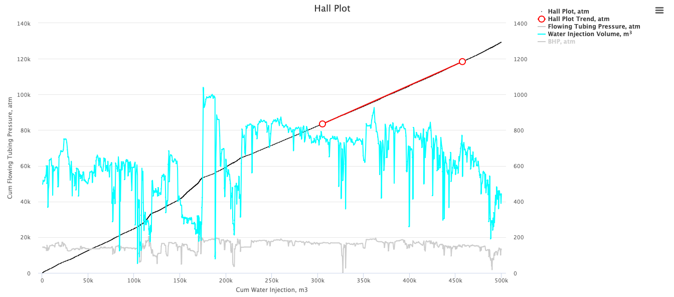
Hall Plot uses readily available Well flowing data: injection rate and wellhead pressures.
The interpretation technique is fitting the data points with the straight lines to estimate injectivity change.
Hall Plot is available online at E&P Portal.
Math & Physics
From Darcy's law for an unfractured injection well located in the center of a circular drainage area, the injection rate in pseudo-steady state is:

Hall integrated both sides with respect to time [2]:

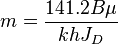
The Cartesian graph of cumulative  versus cumulative injection yields a straight line with slope:
and Injectivity index is:

Hall Plot Application with Wellhead Pressure
Since bottomhole and reservoir pressures are not readily available, the Hall Plot can be used with tubing head pressure.
Given:

Rearranging above:

Under the assumption that the reservoir pressure, friction and gravity terms are constant, a plot of cumulative tubing head pressure versus cumulative injection will yield a straight line. The slope of this line represents the apparent injectivity, which includes the effects of friction, gravity, and reservoir pressure.
Discussion
The Hall Plot is primarily used for qualitative analysis of injectivity changes. A change in slope may indicate:
- Increasing slope indicates formation damage, scaling, increasing skin, or external radius decrease.
- Decreasing slope indicates stimulation, fracturing, increasing water relative permeability (e.g., with surfactant), or increasing well radius (e.g., with acid).
- Constant slope indicates constant skin, reservoir pressure, wellbore radius, external radius and permeability-thickness (kh).
Early in the life of a waterflood, the Hall Plot may exhibit a concave upward appearance. This is caused by the expansion of the external drainage radius and increase in reservoir pressure [3].
The tubing head pressure plot serves as a first-step diagnostic. Any slope changes observed should be verified with a cumulative  versus cumulative
  plot for confirmation.
Multiple wells can be plotted on the same Hall Plot for comparison. This allows for easy identification of wells that are underperforming or responding to stimulation.

Nomenclature
 = formation volume factor, bbl/stb
 = injectivity index, stb/d/psia
 = dimensionless injectivity index, dimensionless
 = permeability times thickness, md·ft
 = slope of Hall Plot, psia·d/bbl
 = bottomhole flowing pressure, psia
 = average reservoir pressure, psia
 = tubing head pressure, psia
- = injection rate, stb/d
 = wellbore radius, ft
 = external drainage radius, ft
 = skin factor, dimensionless
 = frictional pressure drop, psia
 = hydrostatic pressure drop, psia
Greek symbols
 = viscosity, cp
 = time step, days/months
References
- ↑ Hall, H.N. (1963). "How To Analyze Waterflood Injection Well Performance". World Oil.
- ↑ Buell, R.S.; Kazemi, H.; Poettmann, F.H. (1990). "Analyzing Injectivity of Polymer Solutions With the Hall Plot". SPE Reservoir Engineering. 5 (1). doi:10.2118/16963-PA.
- ↑ Wolcott, Don (2009). Applied Waterflood Field Development. Houston: Energy Tribune Publishing Inc.