Difference between revisions of "Hagedorn and Brown correlation"
| (52 intermediate revisions by the same user not shown) | |||
| Line 1: | Line 1: | ||
__TOC__ | __TOC__ | ||
== Brief == | == Brief == | ||
| − | [[Hagedorn and Brown]] is an empirical two-phase flow correlation published in '''1965''' <ref name=HB />. | + | [[Hagedorn and Brown correlation |Hagedorn and Brown]] is an empirical two-phase flow correlation published in '''1965''' <ref name=HB />. |
It doesn't distinguish between the flow regimes. | It doesn't distinguish between the flow regimes. | ||
| − | The heart of the [[Hagedorn and Brown]] method is a correlation for the liquid holdup H<sub>L</sub> <ref name=Economides />. | + | The heart of the [[Hagedorn and Brown correlation|Hagedorn and Brown]] method is a correlation for the liquid holdup H<sub>L</sub> <ref name=Economides />. |
| + | |||
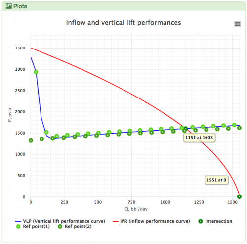
| + | [[Hagedorn and Brown correlation|Hagedorn and Brown]] is the default [[VLP]] correlation for the '''oil wells''' in the [[:Category:PQplot|PQplot]]. | ||
| + | |||
| + | [[File: Hagedorn and Brown.png|thumb|500px|link=https://www.pengtools.com/pqPlot?paramsToken=57e2ad9dd84d56fb56b7515b2ef312bd|Hagedorn and Brown in PQplot Vs Prosper & Kappa |right]] | ||
== Math & Physics == | == Math & Physics == | ||
| Line 21: | Line 25: | ||
== Discussion == | == Discussion == | ||
| − | Why [[Hagedorn and Brown]]? | + | Why [[Hagedorn and Brown correlation| Hagedorn and Brown]]? |
{{Quote| text = One of the consistently best correlations ... | source = Michael Economides et al<ref name=Economides />}} | {{Quote| text = One of the consistently best correlations ... | source = Michael Economides et al<ref name=Economides />}} | ||
| − | + | == Demo == | |
| + | |||
| + | [[Hagedorn and Brown]] correlation overview video: | ||
| + | |||
| + | [[File:Hagedorn and Brown demo.png|400px|https://www.youtube.com/watch?v=DpSv3kWPsIk | Watch on youtube]] | ||
| + | |||
| + | [[Media:Hagedorn and Brown ppt.pdf|Download presentation (pdf)]] | ||
| + | |||
| + | In this video it's shown: | ||
| + | *What the Hagedorn and Brown correlation is | ||
| + | *History and practical application | ||
| + | *Math & Physics | ||
| + | *Flow diagram to get the VLP curve | ||
| + | *Workflow to find HL | ||
== Flow Diagram == | == Flow Diagram == | ||
| Line 31: | Line 48: | ||
[[File: HB Block Diagram.png|400px|HB Block Diagram]] | [[File: HB Block Diagram.png|400px|HB Block Diagram]] | ||
| − | == Workflow | + | == Workflow H<sub>L</sub> == |
| − | |||
| − | |||
:<math> M =SG_o\ 350.52\ \frac{1}{1+WOR}+SG_w\ 350.52\ \frac{WOR}{1+WOR}+SG_g\ 0.0764\ GLR</math><ref name="HB" /> | :<math> M =SG_o\ 350.52\ \frac{1}{1+WOR}+SG_w\ 350.52\ \frac{WOR}{1+WOR}+SG_g\ 0.0764\ GLR</math><ref name="HB" /> | ||
| Line 51: | Line 66: | ||
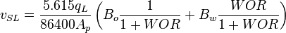
:<math> v_{SL} = \frac{5.615 q_L}{86400 A_p} \left ( B_o \frac{1}{1+WOR} + B_w \frac{WOR}{1+WOR} \right )</math><ref name= Lyons/> | :<math> v_{SL} = \frac{5.615 q_L}{86400 A_p} \left ( B_o \frac{1}{1+WOR} + B_w \frac{WOR}{1+WOR} \right )</math><ref name= Lyons/> | ||
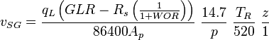
| − | :<math> v_{SG} = \frac{q_L \left ( GLR-R_s \left( \frac{1}{1+WOR}\right) \right )}{86400 A_p}\ \frac{14.7}{p}\ \frac{ | + | :<math> v_{SG} = \frac{q_L \left ( GLR-R_s \left( \frac{1}{1+WOR}\right) \right )}{86400 A_p}\ \frac{14.7}{p}\ \frac{T_R}{520}\ \frac{z}{1}</math><ref name= Lyons/> |
:<math> N_{LV} = 1.938\ v_{SL}\ \sqrt[4]{\frac{\rho_L}{\sigma_L}} </math><ref name= HB/> | :<math> N_{LV} = 1.938\ v_{SL}\ \sqrt[4]{\frac{\rho_L}{\sigma_L}} </math><ref name= HB/> | ||
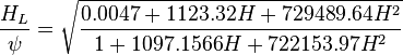
| Line 66: | Line 81: | ||
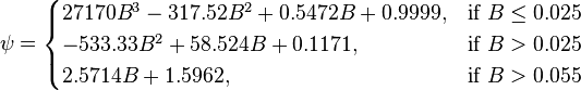
:<math> \psi = \begin{cases} | :<math> \psi = \begin{cases} | ||
| − | 27170 B^3 - 317.52 B^2 + 0.5472 B + 0.9999, &\mbox{if } B | + | 27170 B^3 - 317.52 B^2 + 0.5472 B + 0.9999, &\mbox{if } B \le 0.025 \\ |
-533.33 B^2 + 58.524 B + 0.1171, & \mbox{if }B > 0.025 \\ | -533.33 B^2 + 58.524 B + 0.1171, & \mbox{if }B > 0.025 \\ | ||
2.5714 B +1.5962, & \mbox{if }B > 0.055 | 2.5714 B +1.5962, & \mbox{if }B > 0.055 | ||
| Line 77: | Line 92: | ||
1. Use the no-slip holdup when the original empirical correlation predicts a liquid holdup H<sub>L</sub> less than the no-slip holdup <ref name = Economides/>. | 1. Use the no-slip holdup when the original empirical correlation predicts a liquid holdup H<sub>L</sub> less than the no-slip holdup <ref name = Economides/>. | ||
| − | 2. Use | + | 2. Use the [[Griffith correlation]] to define the bubble flow regime<ref name = Economides/> and calculate H<sub>L</sub>. |
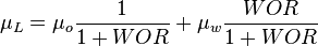
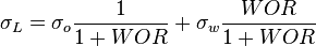
| − | 3. Use watercut instead of WOR to account for the watercut = 100%. | + | 3. Use [[WCUT| watercut]] instead of [[WOR]] to account for the watercut = 100%. |
== Nomenclature == | == Nomenclature == | ||
| + | :<math> A_p </math> = flow area, ft2 | ||
:<math> B </math> = correlation group, dimensionless | :<math> B </math> = correlation group, dimensionless | ||
:<math> B </math> = formation factor, bbl/stb | :<math> B </math> = formation factor, bbl/stb | ||
| Line 89: | Line 105: | ||
:<math> h </math> = depth, ft | :<math> h </math> = depth, ft | ||
:<math> H </math> = correlation group, dimensionless | :<math> H </math> = correlation group, dimensionless | ||
| − | :<math> H_L </math> = liquid holdup factor, | + | :<math> H_L </math> = liquid holdup factor, fraction |
:<math> f </math> = friction factor, dimensionless | :<math> f </math> = friction factor, dimensionless | ||
:<math> GLR </math> = gas-liquid ratio, scf/bbl | :<math> GLR </math> = gas-liquid ratio, scf/bbl | ||
:<math> M </math> = total mass of oil, water and gas associated with 1 bbl of liquid flowing into and out of the flow string, lb<sub>m</sub>/bbl | :<math> M </math> = total mass of oil, water and gas associated with 1 bbl of liquid flowing into and out of the flow string, lb<sub>m</sub>/bbl | ||
| − | :<math> N_D </math> = pipe diameter | + | :<math> N_D </math> = pipe diameter number, dimensionless |
:<math> N_GV </math> = gas velocity number, dimensionless | :<math> N_GV </math> = gas velocity number, dimensionless | ||
:<math> N_L </math> = liquid viscosity number, dimensionless | :<math> N_L </math> = liquid viscosity number, dimensionless | ||
:<math> N_LV </math> = liquid velocity number, dimensionless | :<math> N_LV </math> = liquid velocity number, dimensionless | ||
:<math> p </math> = pressure, psia | :<math> p </math> = pressure, psia | ||
| − | :<math> q_c </math> = conversion constant equal to 32. | + | :<math> q_c </math> = conversion constant equal to 32.174049, lb<sub>m</sub>ft / lb<sub>f</sub>sec<sup>2</sup> |
| − | :<math> | + | :<math> q </math> = total liquid production rate, bbl/d |
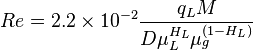
:<math> Re </math> = Reynolds number, dimensionless | :<math> Re </math> = Reynolds number, dimensionless | ||
:<math> R_s </math> = solution gas-oil ratio, scf/stb | :<math> R_s </math> = solution gas-oil ratio, scf/stb | ||
| Line 111: | Line 127: | ||
:<math> \varepsilon </math> = absolute roughness, ft | :<math> \varepsilon </math> = absolute roughness, ft | ||
| − | :<math> \mu </math> = | + | :<math> \mu </math> = viscosity, cp |
:<math> \rho </math> = density, lb<sub>m</sub>/ft<sup>3</sup> | :<math> \rho </math> = density, lb<sub>m</sub>/ft<sup>3</sup> | ||
| − | :<math> \bar \rho </math> = integrated average density at flowing conditions, lb<sub>m</sub>/ft<sup> | + | :<math> \bar \rho </math> = integrated average density at flowing conditions, lb<sub>m</sub>/ft<sup>3</sup> |
| − | :<math> \sigma </math> = surface tension of liquid-air interface, dynes/cm | + | :<math> \sigma </math> = surface tension of liquid-air interface, dynes/cm (ref. values: 72 - water, 35 - oil) |
:<math> \psi </math> = secondary correlation factor, dimensionless | :<math> \psi </math> = secondary correlation factor, dimensionless | ||
===Subscripts=== | ===Subscripts=== | ||
| − | g = gas<BR/> | + | :g = gas<BR/> |
| − | K = °K<BR/> | + | :K = °K<BR/> |
| − | L = liquid<BR/> | + | :L = liquid<BR/> |
| − | o = oil<BR/> | + | :m = gas/liquid mixture<BR/> |
| − | R = °R<BR/> | + | :o = oil<BR/> |
| − | SL = superficial liquid<BR/> | + | :R = °R<BR/> |
| − | SG = superficial gas<BR/> | + | :SL = superficial liquid<BR/> |
| − | w = water<BR/> | + | :SG = superficial gas<BR/> |
| + | :w = water<BR/> | ||
== References == | == References == | ||
| Line 137: | Line 154: | ||
|title=Experimental study of pressure gradients occurring during continuous two-phase flow in small-diameter vertical conduits | |title=Experimental study of pressure gradients occurring during continuous two-phase flow in small-diameter vertical conduits | ||
|journal=Journal of Petroleum Technology | |journal=Journal of Petroleum Technology | ||
| + | |number=SPE-940-PA | ||
|date=1965 | |date=1965 | ||
|volume=17(04) | |volume=17(04) | ||
|pages=475-484 | |pages=475-484 | ||
| + | |url=https://www.onepetro.org/journal-paper/SPE-940-PA | ||
| + | |url-access=registration | ||
}}</ref> | }}</ref> | ||
| Line 202: | Line 222: | ||
[[Category:pengtools]] | [[Category:pengtools]] | ||
| − | [[Category: | + | [[Category:PQplot]] |
| + | |||
| + | {{#seo: | ||
| + | |title=Hagedorn and Brown correlation | ||
| + | |titlemode= replace | ||
| + | |keywords=Hagedorn and Brown, correlation, equation, flow rate, fluids flow, Reynolds number, liquid hold up | ||
| + | |description=Hagedorn and Brown correlation used to calculate reservoir inflow performance curve for nodal analysis | ||
| + | }} | ||
Latest revision as of 12:21, 1 November 2018
Contents
Brief
Hagedorn and Brown is an empirical two-phase flow correlation published in 1965 [1].
It doesn't distinguish between the flow regimes.
The heart of the Hagedorn and Brown method is a correlation for the liquid holdup HL [2].
Hagedorn and Brown is the default VLP correlation for the oil wells in the PQplot.
Math & Physics
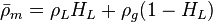
Following the law of conservation of energy the basic steady state flow equation is:
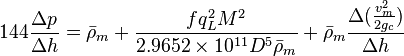
where
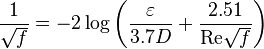
Colebrook–White [3] equation for the Darcy's friction factor:
Reynolds two phase number:
Discussion
Why Hagedorn and Brown?
One of the consistently best correlations ...— Michael Economides et al[2]
Demo
Hagedorn and Brown correlation overview video:

In this video it's shown:
- What the Hagedorn and Brown correlation is
- History and practical application
- Math & Physics
- Flow diagram to get the VLP curve
- Workflow to find HL
Flow Diagram

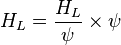
Workflow HL


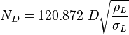
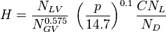
![N_L = 0.15726\ \mu_L \sqrt[4]{\frac{1}{\rho_L \sigma_L^3}}](/images/math/b/2/0/b207fe79b4a4ee53d466e182791ca737.png)

![N_{LV} = 1.938\ v_{SL}\ \sqrt[4]{\frac{\rho_L}{\sigma_L}}](/images/math/d/d/8/dd824df0b6ec22aa724161b929e993fe.png)
![N_{GV} = 1.938\ v_{SG}\ \sqrt[4]{\frac{\rho_L}{\sigma_L}}](/images/math/3/6/4/364153c39c1657b3b7bab8f7ed710e60.png)
Modifications
1. Use the no-slip holdup when the original empirical correlation predicts a liquid holdup HL less than the no-slip holdup [2].
2. Use the Griffith correlation to define the bubble flow regime[2] and calculate HL.
3. Use watercut instead of WOR to account for the watercut = 100%.
Nomenclature
 = flow area, ft2
 = correlation group, dimensionless
- = formation factor, bbl/stb
 = coefficient for liquid viscosity number, dimensionless
 = pipe diameter, ft
 = depth, ft
 = correlation group, dimensionless
 = liquid holdup factor, fraction
 = friction factor, dimensionless
 = gas-liquid ratio, scf/bbl
 = total mass of oil, water and gas associated with 1 bbl of liquid flowing into and out of the flow string, lbm/bbl
 = pipe diameter number, dimensionless
 = gas velocity number, dimensionless
 = liquid viscosity number, dimensionless
 = liquid velocity number, dimensionless
 = pressure, psia
 = conversion constant equal to 32.174049, lbmft / lbfsec2
 = total liquid production rate, bbl/d
 = Reynolds number, dimensionless
 = solution gas-oil ratio, scf/stb
 = specific gravity, dimensionless
 = temperature, °R or °K, follow the subscript
 = velocity, ft/sec
 = water-oil ratio, bbl/bbl
 = gas compressibility factor, dimensionless
Greek symbols
 = absolute roughness, ft
 = viscosity, cp
 = density, lbm/ft3
 = integrated average density at flowing conditions, lbm/ft3
 = surface tension of liquid-air interface, dynes/cm (ref. values: 72 - water, 35 - oil)
 = secondary correlation factor, dimensionless
Subscripts
- g = gas
- K = °K
- L = liquid
- m = gas/liquid mixture
- o = oil
- R = °R
- SL = superficial liquid
- SG = superficial gas
- w = water
References
- ↑ 1.0 1.1 1.2 1.3 1.4 1.5 1.6 1.7 1.8 1.9 Hagedorn, A. R.; Brown, K. E. (1965). "Experimental study of pressure gradients occurring during continuous two-phase flow in small-diameter vertical conduits"
 . Journal of Petroleum Technology. 17(04) (SPE-940-PA): 475–484.
- ↑ 2.0 2.1 2.2 2.3 2.4 2.5 2.6 Economides, M.J.; Hill, A.D.; Economides, C.E.; Zhu, D. (2013). Petroleum Production Systems (2 ed.). Westford, Massachusetts: Prentice Hall. ISBN 978-0-13-703158-0.
- ↑ Colebrook, C. F. (1938–1939). "Turbulent Flow in Pipes, With Particular Reference to the Transition Region Between the Smooth and Rough Pipe Laws"
 . Journal of the Institution of Civil Engineers. London, England. 11: 133–156.
- ↑ Moody, L. F. (1944). "Friction factors for pipe flow". Transactions of the ASME. 66 (8): 671–684.
- ↑ 5.0 5.1 5.2 5.3 5.4 5.5 Lyons, W.C. (1996). Standard handbook of petroleum and natural gas engineering. 2. Houston, TX: Gulf Professional Publishing. ISBN 0-88415-643-5.
- ↑ 6.0 6.1 Trina, S. (2010). An integrated horizontal and vertical flow simulation with application to wax precipitation (Master of Engineering Thesis). Canada: Memorial University of Newfoundland.