Difference between revisions of "Category: FracDesign"
From wiki.pengtools.com
(→Pumping schedule) |
(→Pumping schedule) |
||
| Line 102: | Line 102: | ||
:<math>c_{stage} = \frac {\int \limits_{t_{start}}^{t_{end}} c_e \left ( \frac{t-t_{pad}}{t_e-t_{pad}} \right )^{\epsilon} dt}{t_{end}-t_{start}} </math> - ramping stage slurry concentration | :<math>c_{stage} = \frac {\int \limits_{t_{start}}^{t_{end}} c_e \left ( \frac{t-t_{pad}}{t_e-t_{pad}} \right )^{\epsilon} dt}{t_{end}-t_{start}} </math> - ramping stage slurry concentration | ||
| − | :<math>c_a=\frac{c}{ | + | :<math>c_a=\frac{c}{1-\frac{c}{\rho_p}}</math> - conversion form slurry concentration (proppant mass per unit of injected slurry) to clean concentration (proppant mass per unit of injected clean (base, "neat") fluid) |
==References== | ==References== | ||
Revision as of 07:43, 10 October 2018
Contents
Brief
fracDesign is a tool for designing a hydraulic fracture treatment in pengtools.
For the given set of reservoir, fluid and proppant properties fracDesign calculates the pumping schedule which will create the optimal fracture geometry to achieve maximum well’s productivity.
fracDesignis available online at www.pengtools.com.
Main features
- PKN and KGD fracture geometry models
- optiFrac workflow on fracture geometry optimization
- Slurry concentration versus time pumping schedule as plot and table
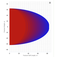
- Fracture length and width profiles vs time plots
- Net pressure profiles vs time as plot and table
- Practical pumping constrains and Fracture tuning options
- Detailed output table with calculated fracture design parameters
- Sensitivity option with benchmark to potential
- Simulation mode: calculating the fracture geometry from the given pumping schedule
Interface features
- "Default values" button resets input values to the default values.
- Switch between Metric and Field units.
- Save/load models to the files and to the user’s cloud.
- Export pdf report containing input parameters, calculated values and the chart.
- Share models to the public cloud or by using model’s link.
- Continue your work from where you stopped: last saved model will be automatically opened.
- Download the chart as an image or data and print (upper-right corner chart’s button).
Math & Physics
 - hydraulic maximum fracture width PKN (ref[1] eq 9.53)
 - hydraulic maximum fracture width KGD (ref[1] eq 9.55)
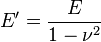 - plain strain modulus
 - hydraulic average fracture width
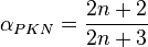
 - shape factor PKN (ref[1] eq 9.10)
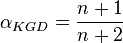
 - shape factor KGD (ref[1] eq 9.24)
 - mass balance equation (ref[1] eq 8.1)
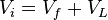
 - injected volume into one fracture wing
 - the area of one face of one wing for rectangular fracture shape
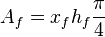 - the area of one face of one wing for elliptic fracture shape
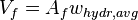 - volume of fluid contained in one fracture wing
 - volume of fluid leak-off to formation through the two created fracture surfaces of one wing
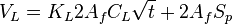
 - mass balance equation (ref[2] eq 4.6)
 - fluid efficiency
Opening time distribution factor KL
Nolte opening time distribution factor KL
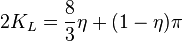 - (ref[1] eq 8.36)
Carter opening time distribution factor KL
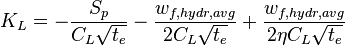 (ref [2] eq 4.8)
where:
 (ref [2] eq 4.9)
and:
 (ref [2] eq 4.9)
Nolte G-function for opening time distribution factor KL
 (ref [2] eq 4.12)
where:
Pumping schedule
 - Nolte exponent
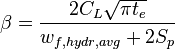
 - pad pumping time
 - proppant concentration at the end of pumping
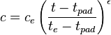 - slurry concentration vs time
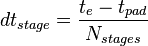 - ramping stage duration
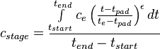 - ramping stage slurry concentration
 - conversion form slurry concentration (proppant mass per unit of injected slurry) to clean concentration (proppant mass per unit of injected clean (base, "neat") fluid)
References
- ↑ 1.0 1.1 1.2 1.3 1.4 1.5 Valko, Peter; Economides, Michael J. (1995). Hydraulic fracture mechanics. Texas A & M University: John Wiley and Sons.
- ↑ 2.0 2.1 2.2 2.3 2.4 Economides, Michael J.; Oligney, Ronald; Valko, Peter (2002). Unified Fracture Design: Bridging the Gap Between Theory and Practice. Alvin, Texas: Orsa Press.
Pages in category "FracDesign"
The following 8 pages are in this category, out of 8 total.