Hagedorn and Brown correlation
Contents
Brief
Hagedorn and Brown is an empirical two-phase flow correlation published in 1965.
It doesn't distinguish between the flow regimes.
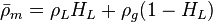
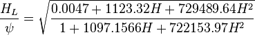
The heart of the Hagedorn and Brown method is a correlation for the liquid holdup  .
.
Math & Physics
Following the law of conservation of energy the basic steady state flow equation is:
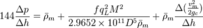
where
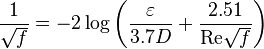
Colebrook–White equation for the Darcy's friction factor:
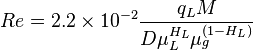
Reynolds two phase number:
Discussion
Flow Diagram

Workflow
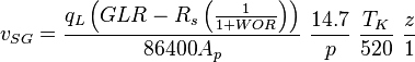
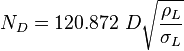
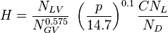
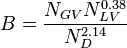
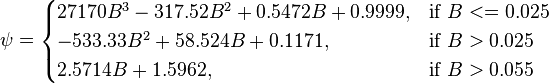
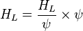
To find calculate:


![N_L = 0.15726\ \mu_L \sqrt[4]{\frac{1}{\rho_L \sigma_L^3}}](/images/math/b/2/0/b207fe79b4a4ee53d466e182791ca737.png)

![N_{LV} = 1.938\ v_{SL}\ \sqrt[4]{\frac{\rho_L}{\sigma_L}}](/images/math/d/d/8/dd824df0b6ec22aa724161b929e993fe.png)
![N_{GV} = 1.938\ v_{SG}\ \sqrt[4]{\frac{\rho_L}{\sigma_L}}](/images/math/3/6/4/364153c39c1657b3b7bab8f7ed710e60.png)
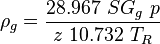
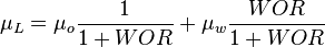
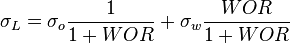
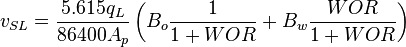
Nomenclature
References
wikipedia.org Darcy friction factor formulae
Economides Production Petroleum Systems
Hagedorn, A. R., & Brown, K. E. (1965). Experimental study of pressure gradients occurring during continuous two-phase flow in small-diameter vertical conduits. Journal of Petroleum Technology, 17(04), 475-484.
Lyons WC. 1996. Standard handbook of petroleum and natural gas engineering. Gulf Publishing Company, Houston, TX.
Guo B, Lyons WC, Chalambor A. 2007. Petroleum production engineering, A computer assisted approach. Elsevier Science & Technology Books
Trina S. 2010. An integrated horizontal and vertical flow simulation with application to wax precipitation. Master of Engineering Thesis, Memorial University of Newfoundland, Canada.
Haaland SE. 1983. Simple and Explicit Formulas for the Friction Factor in Turbulent Pipe Flow. Journal of Fluids Engineering. Vol. 105, pp. 89-90.
- ↑ Moody, L. F. (1944), "Friction factors for pipe flow", Transactions of the ASME, 66 (8): 671–684
- ↑ Colebrook, C. F. (1938–1939). "Turbulent Flow in Pipes, With Particular Reference to the Transition Region Between the Smooth and Rough Pipe Laws". Journal of the Institution of Civil Engineers. London, England. 11: 133–156.