Difference between revisions of "Hagedorn and Brown correlation"
From wiki.pengtools.com
(→Workflow) |
(→Workflow) |
||
| Line 39: | Line 39: | ||
:<math> CN_L = 0.061\ N_L^3 - 0.0929\ N_L^2 + 0.0505\ N_L + 0.0019 </math> | :<math> CN_L = 0.061\ N_L^3 - 0.0929\ N_L^2 + 0.0505\ N_L + 0.0019 </math> | ||
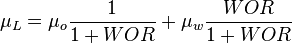
| − | :<math> v_{SL} = \frac{5.615 q_L}{86400 A_p} \left ( B_o | + | :<math> v_{SL} = \frac{5.615 q_L}{86400 A_p} \left ( B_o \frac{1}{1+WOR} + B_w /frac{WOR}{1+WOR} \right )</math> |
:<math> v_{SG} </math> | :<math> v_{SG} </math> | ||
Revision as of 13:33, 21 March 2017
Contents
Brief
Hagedorn and Brown is an empirical two-phase flow correlation published in 1965.
It doesn't distinguish between the flow regimes.
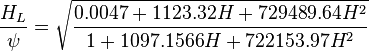
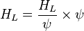
The heart of the Hagedorn and Brown method is a correlation for the liquid holdup : .
.
Math & Physics
Following the law of conservation of energy the basic steady state flow equation is:
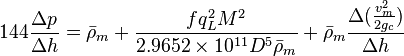
where
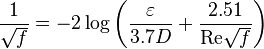
Colebrook–White equation for the Darcy's friction factor:
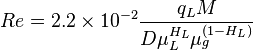
Reynolds two phase number:


![N_L = 0.15726\ \mu_L \sqrt[4]{\frac{1}{\rho_L \sigma_L^3}}](/images/math/b/2/0/b207fe79b4a4ee53d466e182791ca737.png)


![N_{LV} = 1.938\ v_{SL}\ \sqrt[4]{\frac{\rho_L}{\sigma}}](/images/math/2/f/2/2f2abb2b5e504663beb5ddb87301af09.png)
![N_{GV} = 1.938\ v_{SG}\ \sqrt[4]{\frac{\rho_L}{\sigma}}](/images/math/4/0/c/40cab20a6f3a6a92f320bbff38c696cd.png)