Difference between revisions of "Hagedorn and Brown correlation"
From wiki.pengtools.com
(→Nomenclature) |
(→Nomenclature) |
||
| Line 100: | Line 100: | ||
:<math> \mu_L </math> = liquid viscosity, cp | :<math> \mu_L </math> = liquid viscosity, cp | ||
:<math> \mu_g </math> = gas viscosity, cp | :<math> \mu_g </math> = gas viscosity, cp | ||
| + | :<math> \mu_o </math> = oil viscosity, cp | ||
| + | :<math> SG_o </math> = oil specific gravity, dimensionless | ||
| + | :<math> SG_w </math> = water specific gravity, dimensionless | ||
| + | :<math> SG_g </math> = gas specific gravity, dimensionless | ||
| + | :<math> WOR </math> = water-oil ratio, bbl/bbl | ||
| + | :<math> GLR </math> = gas-liquid ratio, scf/bbl | ||
| + | :<math> R_s </math> = solution gas-oil ratio, scf/stb | ||
| + | :<math> z </math> = gas compressibility factor, dimensionless | ||
| + | :<math> T_R </math> = temperature, °R | ||
| + | :<math> \sigma_L </math> = surface tension of liquid-air interface, dynes/cm | ||
| + | :<math> \sigma_o </math> = surface tension of liquid-oil interface, dynes/cm | ||
| + | :<math> \sigma_w </math> = surface tension of liquid-water interface, dynes/cm | ||
== References == | == References == | ||
Revision as of 12:46, 24 March 2017
Contents
Brief
Hagedorn and Brown is an empirical two-phase flow correlation published in 1965 [1].
It doesn't distinguish between the flow regimes.
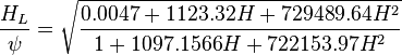
The heart of the Hagedorn and Brown method is a correlation for the liquid holdup  [2].
[2].
Math & Physics
Following the law of conservation of energy the basic steady state flow equation is:
where
Colebrook–White [3] equation for the Darcy's friction factor:
Reynolds two phase number:
Discussion
Why Hagedorn and Brown?
The of the consistently best correlations was found to be the empirical Hagedorn and Brown correlation.— Economides
Cry "Havoc" and let slip the dogs of war.— William Shakespeare, Julius Caesar, act III, scene I
One of the consistently best correlations was found to be the empirical Hagedorn and Brown correlation. [2]
Flow Diagram

Workflow
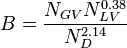
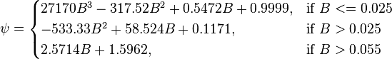
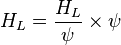
To find calculate:


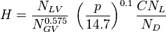
![N_L = 0.15726\ \mu_L \sqrt[4]{\frac{1}{\rho_L \sigma_L^3}}](/images/math/b/2/0/b207fe79b4a4ee53d466e182791ca737.png)

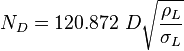
![N_{LV} = 1.938\ v_{SL}\ \sqrt[4]{\frac{\rho_L}{\sigma_L}}](/images/math/d/d/8/dd824df0b6ec22aa724161b929e993fe.png)
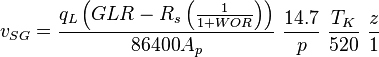
![N_{GV} = 1.938\ v_{SG}\ \sqrt[4]{\frac{\rho_L}{\sigma_L}}](/images/math/3/6/4/364153c39c1657b3b7bab8f7ed710e60.png)
Nomenclature
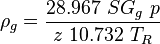
 = pressure, psia
 = depth, ft
- = liquid holdup factor, dimensionless
 = average mixture destiny at flowing conditions, lbm/ft2
 = friction factor, dimensionless
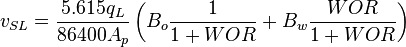
 = total liquid production rate, bbl/d
 = total mass of oil, water and gas associated with 1 bbl of liquid flowing into and out of the flow string, lbm/bbl
 = pipe diameter, ft
 = mixture velocity, ft/sec
 = conversion constant equal to 32.174, lbmft / lbfsec2
 = liquid destiny, lbm/ft2
 = gas destiny, lbm/ft2
 = absolute roughness, ft
 = Reynolds number, dimensionless
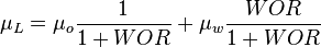
 = liquid viscosity, cp
 = gas viscosity, cp
 = oil viscosity, cp
 = oil specific gravity, dimensionless
 = water specific gravity, dimensionless
 = gas specific gravity, dimensionless
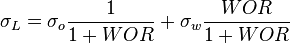
 = water-oil ratio, bbl/bbl
 = gas-liquid ratio, scf/bbl
 = solution gas-oil ratio, scf/stb
 = gas compressibility factor, dimensionless
 = temperature, °R
 = surface tension of liquid-air interface, dynes/cm
 = surface tension of liquid-oil interface, dynes/cm
 = surface tension of liquid-water interface, dynes/cm
References
- ↑ 1.0 1.1 1.2 1.3 1.4 1.5 1.6 1.7 1.8 1.9 Hagedorn, A. R.; Brown, K. E. (1965). "Experimental study of pressure gradients occurring during continuous two-phase flow in small-diameter vertical conduits". Journal of Petroleum Technology. 17(04): 475–484.
- ↑ 2.0 2.1 2.2 2.3 2.4 Economides, M.J.; Hill, A.D.; Economides, C.E.; Zhu, D. (2013). Petroleum Production Systems (2 ed.). Westford, Massachusetts: Prentice Hall. ISBN 978-0-13-703158-0.
- ↑ Colebrook, C. F. (1938–1939). "Turbulent Flow in Pipes, With Particular Reference to the Transition Region Between the Smooth and Rough Pipe Laws"
 . Journal of the Institution of Civil Engineers. London, England. 11: 133–156.
- ↑ Moody, L. F. (1944). "Friction factors for pipe flow". Transactions of the ASME. 66 (8): 671–684.
- ↑ 5.0 5.1 5.2 5.3 5.4 5.5 Lyons, W.C. (1996). Standard handbook of petroleum and natural gas engineering. 2. Houston, TX: Gulf Professional Publishing. ISBN 0-88415-643-5.
- ↑ 6.0 6.1 Trina, S. (2010). An integrated horizontal and vertical flow simulation with application to wax precipitation (Master of Engineering Thesis). Canada: Memorial University of Newfoundland.