Difference between revisions of "Hagedorn and Brown correlation"
From wiki.pengtools.com
(→Discussion) |
(→Discussion) |
||
| Line 23: | Line 23: | ||
Why [[Hagedorn and Brown]]? | Why [[Hagedorn and Brown]]? | ||
| − | ''One of the consistently best correlations was found to be the empirical Hagedorn and Brown correlation.'' <ref = Economides | + | ''One of the consistently best correlations was found to be the empirical Hagedorn and Brown correlation.'' <ref name=Economides />. |
== Flow Diagram == | == Flow Diagram == | ||
Revision as of 12:05, 24 March 2017
Contents
Brief
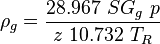
Hagedorn and Brown is an empirical two-phase flow correlation published in 1965 [1].
It doesn't distinguish between the flow regimes.
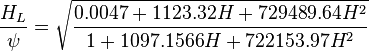
The heart of the Hagedorn and Brown method is a correlation for the liquid holdup  [2].
[2].
Math & Physics
Following the law of conservation of energy the basic steady state flow equation is:
where
Colebrook–White [3] equation for the Darcy's friction factor:
Reynolds two phase number:
Discussion
Why Hagedorn and Brown?
One of the consistently best correlations was found to be the empirical Hagedorn and Brown correlation. [2].
Flow Diagram

Workflow
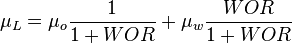
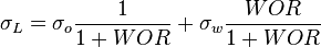
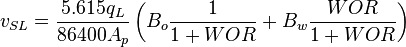
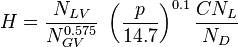
To find calculate:


![N_L = 0.15726\ \mu_L \sqrt[4]{\frac{1}{\rho_L \sigma_L^3}}](/images/math/b/2/0/b207fe79b4a4ee53d466e182791ca737.png)

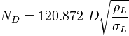
![N_{LV} = 1.938\ v_{SL}\ \sqrt[4]{\frac{\rho_L}{\sigma_L}}](/images/math/d/d/8/dd824df0b6ec22aa724161b929e993fe.png)
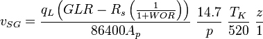
![N_{GV} = 1.938\ v_{SG}\ \sqrt[4]{\frac{\rho_L}{\sigma_L}}](/images/math/3/6/4/364153c39c1657b3b7bab8f7ed710e60.png)
Nomenclature
References
- ↑ 1.0 1.1 1.2 1.3 1.4 1.5 1.6 1.7 1.8 1.9 Hagedorn, A. R.; Brown, K. E. (1965). "Experimental study of pressure gradients occurring during continuous two-phase flow in small-diameter vertical conduits". Journal of Petroleum Technology. 17(04): 475–484.
- ↑ 2.0 2.1 2.2 2.3 2.4 Economides, M.J.; Hill, A.D.; Economides, C.E.; Zhu, D. (2013). Petroleum Production Systems (2 ed.). Westford, Massachusetts: Prentice Hall. ISBN 978-0-13-703158-0.
- ↑ Colebrook, C. F. (1938–1939). "Turbulent Flow in Pipes, With Particular Reference to the Transition Region Between the Smooth and Rough Pipe Laws"
 . Journal of the Institution of Civil Engineers. London, England. 11: 133–156.
- ↑ Moody, L. F. (1944). "Friction factors for pipe flow". Transactions of the ASME. 66 (8): 671–684.
- ↑ 5.0 5.1 5.2 5.3 5.4 5.5 Lyons, W.C. (1996). Standard handbook of petroleum and natural gas engineering. 2. Houston, TX: Gulf Professional Publishing. ISBN 0-88415-643-5.
- ↑ 6.0 6.1 Trina, S. (2010). An integrated horizontal and vertical flow simulation with application to wax precipitation (Master of Engineering Thesis). Canada: Memorial University of Newfoundland.